Dharani Suresh

🛰️🌍 Data from Above, Delve and Discover: Unveiling Earth’s Veil with NASA’s Tools 🛰️🌍

– Developed By Dharani

Welcome to a journey through the vast expanse of Earth’s data landscapes, where cutting-edge technology meets the open frontiers of science! In this guide, you’ll dive into the powerful interfaces of APIs, including NASA’s AρρEEARS platform, to retrieve and manipulate satellite data that illuminate our understanding of the planet. This page is your gateway to mastering the art of data-driven discoveries in environmental and climate research. Prepare to unlock the secrets of the Earth through:

🔁 Open and Reproducible Science: Reproducible research practices using APIs.

🛰️ Dynamic Data Retrieval: Harness APIs to access real-time satellite observations.

🌱 Green Insights with NDVI and EVI: Track and analyze the vitality of Earth’s vegetation.

💡 Tech Exploration: Navigate through an array of python libraries and fuctions enhancing Earth science.

🗺️ Mapping Mastery: Integrate OpenStreetMap to enrich your data overlays.

📐 Precise Data Clipping: Focus your studies with pinpoint geographical accuracy.

🌍 Interpreting Earth’s Palette: Decode environmental changes through visual data.

Whether you’re a seasoned scientist, an enthusiastic educator, or a curious student, these insights offer a starting point for anyone eager to explore the interplay of technology and nature. Let’s embark on this educational adventure together, unlocking the power of open data and reproducible science to make a lasting impact on our understanding of the world around us.

Open and Reproducible Science Image Source: Earthdata

Open Science

Open science is the movement to make scientific research, data, and dissemination accessible to all. This approach promotes transparency, accelerates innovation, and strengthens the credibility of research findings.

Reproducible Science

Reproducible science ensures that scientific experiments can be consistently repeated and verified by other researchers. It involves sharing the code, data, and methods used in research to promote transparency and reliability.

Introduction to API

Image Source: API

What is an API?

An API, or Application Programming Interface, is a set of rules and protocols for building and interacting with software applications. APIs allow different software systems to communicate with each other, enabling functionalities to be abstracted and reused efficiently.

In Simple Words: Imagine you have a magic notebook. Whenever you write a question in it, it sends the question to a magical library where all sorts of information are kept. The library finds the answer and writes it back in your notebook. An API works like that notebook—it sends your questions (requests) to a computer system that has lots of data, and then it brings the answers back to you.

Uses and Benefits of APIs

APIs are crucial for creating flexible, modular software applications. They allow developers to use functionalities provided by other services without understanding the intricate details of their implementation. This modularity makes development faster, more secure, and more scalable. Additionally, APIs enable dynamic interactions between different software components, enhancing real-time data exchange and responsiveness in applications.

Types of APIs

APIs come in various types, each designed to facilitate different kinds of interactions between software applications. Here’s a breakdown of the primary types of Web APIs commonly used in technology: Web APIs (Also known as Web Services), Open APIs (Also known as Public APIs), Internal APIs (Also referred to as Private APIs), Partner APIs, Composite APIs, Database APIs, Hardware APIs, Content Management APIs, Payment APIs, Social Media APIs. In this material, the focus is particularly on Web APIs, especially RESTful APIs.

Types of Web APIs

Web APIs are designed to be accessed over the web using HTTP protocols. They allow for interaction between different software systems over the internet. They are commonly categorized into:

• RESTful APIs (Representational State Transfer): Uses standard HTTP methods like GET, POST, PUT, DELETE. They are stateless and can return data in various formats such as JSON, XML, or YAML.
• SOAP APIs (Simple Object Access Protocol): Uses XML for messaging and requires more extensive setup and overhead but is considered highly secure and robust.
• GraphQL: Allows clients to request exactly the data they need, making it efficient especially for complex systems with many interrelated resources.

Example of Web APIs Applications

• Weather Monitoring: APIs access real-time weather data from global meteorological sources, enabling apps and websites to display current conditions, forecasts, and severe weather alerts.
• Accessing Satellite Images: APIs provide access to up-to-date satellite imagery and geospatial data, crucial for applications in environmental monitoring, disaster response, and urban planning.
• Online Shopping Platforms: APIs facilitate the integration of product listings, payment gateways, and shipping logistics, enhancing user experience by streamlining e-commerce operations and enabling personalized shopping recommendations.

Overview of NASA Earth Data’s AρρEEARS API

The “AρρEEARS” platform, accessible through the Earthdata website, is an API that enables users to programmatically request, retrieve, and manipulate large datasets from NASA’s Earth observing data. This powerful tool provides a set of predefined protocols and utilities that facilitate the integration of AρρEEARS into applications or scripts, automating tasks like data extraction and analysis. By leveraging NASA’s extensive data repositories, AρρEEARS supports a wide range of environmental research and educational applications.

Key Features of the AρρEEARS Platform

• Single Interface for Multiple Data Collections: Users can access a variety of geospatial data from numerous NASA Earth observation sources through a unified interface. This makes it easier to handle data requests that span multiple data collections.

• Support for Time-Series and Area-Based Extractions: Whether users need data over a specific period or across a particular geographical area, AρρEEARS accommodates both time-series and area-based requests. This flexibility is crucial for comprehensive environmental monitoring and analysis.

• Visualization and Analysis Tools: The platform offers tools that allow users to visualize, analyze, and interpret the requested data within the interface itself. This helps in making informed decisions based on the processed data which is tailored to the user’s specific needs.

• Download Processed Satellite Data: Users can download processed and analysis-ready satellite data, which can be directly used for further scientific studies or educational purposes, significantly simplifying the data acquisition process.

AρρEEARS thus serves as an invaluable resource for researchers, educators, and policy-makers involved in environmental sciences, offering streamlined access to high-quality satellite data and enhancing the efficiency of environmental data management and analysis.

You can explore the complete range of products and tools available on this link: Explore NASA Earthdata’s AρρEEARS Products

The AρρEEARS platform offers a variety of satellite data products, each suited for different research needs. Some of the products include:

• MODIS (Moderate Resolution Imaging Spectroradiometer): Provides data useful for monitoring global dynamics including changes in Earth’s surface and cloud cover. Spatial resolution ranges from 250 meters to 1 kilometer, with a temporal resolution that provides global coverage every 1 to 2 days.
• VIIRS (Visible Infrared Imaging Radiometer Suite): Delivers data for observing weather patterns, natural disasters, and the health of vegetation. It offers a spatial resolution of 375 meters to 750 meters and a temporal resolution providing daily global coverage.
• Landsat: Offers detailed imagery that’s beneficial for studying land use change, forestry, and agriculture. Spatial resolution is about 30 meters for multispectral bands, with panchromatic bands at 15 meters. Temporal resolution sees a complete Earth coverage every 16 days.
• ECOSTRESS: Focuses on plant temperature, providing insights into plant health and water usage. It features a spatial resolution of approximately 70 meters at nadir, with a temporal resolution that varies significantly depending on the International Space Station’s orbit but generally revisits areas every few days.

For a detailed exploration of each satellite product, you can visit the AρρEEARS products page.

Let’s see in action!

This exercise will involve obtaining NDVI and EVI data from MODIS for a location (Finley) in Wisconsin, covering the period between 2020 and 2023. This location features vegetation, agricultural land, and urban settlements. It will be interesting to observe how NDVI and EVI change over this period.

What is NDVI and EVI?

• NDVI (Normalized Difference Vegetation Index): NDVI is a measure of vegetation greenness or density based on the difference in reflectance between near-infrared (NIR) and red light bands captured by satellite sensors. It is widely used to assess the health, density, and productivity of vegetation. In MODIS, NIR is typically captured in band 2.

• EVI (Enhanced Vegetation Index): EVI is an improved version of NDVI that corrects for atmospheric and background noise effects, particularly in areas with dense vegetation. It provides a more accurate representation of vegetation cover and condition compared to NDVI. In MODIS, NIR is typically captured in band 2, red in band 1, and blue in band 3.

Formulas to Calculate NDVI and EVI:

1. NDVI Formula:

   

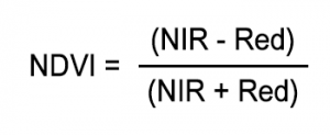
   Where:

   • NIR (Near-Infrared) is the reflectance in MODIS band 2.
   • Red is the reflectance in MODIS band 1.

2. EVI Formula:

   

   Where:

   • NIR (Near-Infrared) is the reflectance in MODIS band 2.
   • Red is the reflectance in MODIS band 1.
   • Blue is the reflectance in MODIS band 3.
   • ( G ) is the gain factor (2.5 by default).
   • ( C1 ) is the coefficient of atmospheric resistance (6 by default).
   • ( C2 ) is the coefficient of canopy background adjustment (7.5 by default).
   • ( L ) is the soil adjustment factor (1 by default).

These indices are calculated using satellite imagery data, where reflectance values are extracted from the corresponding bands. The resulting NDVI and EVI values provide insights into vegetation health, density, and growth.

Source: NASA - MODIS Products: NDVI and (EVI)

Illustration:

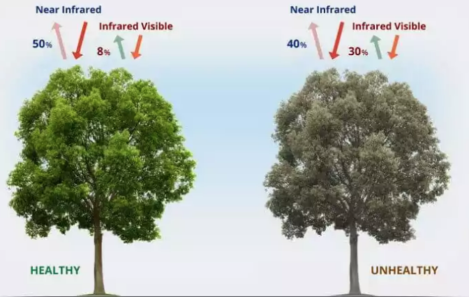
Image Source: Healthy and Stressed Illustration

The above image visually illustrates how the health of vegetation can be discerned through remote sensing techniques using indices such as the NDVI and the EVI. These indices utilize the distinct properties of light absorption and reflection by healthy and unhealthy vegetation to provide quantitative measures of vegetation health.

NDVI Explanation: NDVI takes advantage of the fact that chlorophyll in healthy vegetation absorbs most visible light (mainly red) and reflects a large portion of near-infrared light. In the image:

• Healthy Tree: Shows a high reflection of near-infrared light (50%) and low absorption of visible light (8%), leading to a higher NDVI value. This indicates vigorous photosynthetic activity and, thus, good health.
• Unhealthy Tree: Reflects less near-infrared light (40%) and absorbs more visible light (30%), resulting in a lower NDVI value. This is typical for vegetation under stress, as stressed or diseased plants reflect less NIR light and more visible light due to less chlorophyll and potentially damaged cellular structures.

NDVI values range from -1 to +1, where values close to +1 suggest dense, healthy green vegetation, and values near zero or negative indicate non-vegetative surfaces such as water, rocks, or barren areas.

EVI Explanation: EVI enhances NDVI by correcting distortions in reflected light caused by atmospheric particles and ground cover beneath the vegetation. It is specifically designed to optimize the vegetation signal in high biomass areas and addresses issues where NDVI values saturate.

• Healthy Tree: The higher NIR reflectance and lower visible light absorption would still result in a higher EVI, but the calculation would factor in corrections for atmospheric conditions and background signal noise, providing a more accurate measure of green biomass and canopy structural variations.
• Unhealthy Tree: With higher absorption and lower reflection rates, the EVI would similarly be lower than that of healthy vegetation, but the index would more accurately reflect the true vegetation cover and health, accounting for aerosol influences and background soil reflections.

EVI values also ranges from -1 to +1. Similar to NDVI, positive EVI values indicate the presence of vegetation. High positive values (close to +1) are typical for areas with high-density green vegetation, while values closer to zero or negative values suggest barren, non-vegetative surfaces, or water.

Both NDVI and EVI are critical for monitoring vegetation health via satellite imagery, aiding in environmental management, agriculture, and climate studies by providing data-driven insights into the condition of plant life across the globe. This depiction helps to underscore the physical basis for these indices, emphasizing the difference in light absorption and reflection patterns associated with healthy versus unhealthy vegetation.

Step-by-Step Instructions

Each step in the notebook will be clearly described, providing detailed instructions on how to execute the code, understand the output, and modify parameters for different analyses.

This demonstration has 4 parts:

• 🌍 Part 1: Accessing OpenStreetMap and AppEEARS API
  • Discusses how to access and utilize the OpenStreetMap and AppEEARS API for gathering and analyzing geospatial data.
• 🌱 Part 2: Comparative Analysis of NDVI and EVI
  • Explores the comparison of the sensitivity and responsiveness of NDVI and EVI to different vegetation types or stress conditions.
• 📈 Part 3: Trend Analysis Over Time
  • Examines how to identify changes in vegetation cover over the time period covered by the data.
• 🔍 Part 4: Change Detection and Anomaly Detection Analysis
  • Investigates methods to identify specific areas within the location that have undergone significant changes in vegetation over the four-year period.

### Part 1: Accesing APIs

Objective:This section explains how to access and utilize the OpenStreetMap and AppEEARS API for collecting and analyzing geospatial data. It covers topics such as visualizing geographic boundaries, downloading satellite imagery, and managing and analyzing data.

First, create a login account at Earth Data to access comprehensive Earth observation data. Visit the official NASA Earthdata Login website at https://urs.earthdata.nasa.gov.

This code installs a Python package named EarthPy from a specific GitHub repository using pip. The “@apppears” part refers to a specific branch, tag, or commit of the repository to install.

!pip install git+https://github.com/earthlab/earthpy@apppears

Collecting git+https://github.com/earthlab/earthpy@apppears
  Cloning https://github.com/earthlab/earthpy (to revision apppears) to /tmp/pip-req-build-qt2wuvju
  Running command git clone --filter=blob:none --quiet https://github.com/earthlab/earthpy /tmp/pip-req-build-qt2wuvju
  Running command git checkout -b apppears --track origin/apppears
  Switched to a new branch 'apppears'
  Branch 'apppears' set up to track remote branch 'apppears' from 'origin'.
  Resolved https://github.com/earthlab/earthpy to commit 20e0b17e563da17ba46dc32832cf4ed9173a7531
  Installing build dependencies ... [?25ldone
[?25h  Getting requirements to build wheel ... [?25ldone
[?25h  Preparing metadata (pyproject.toml) ... [?25ldone
[?25hRequirement already satisfied: geopandas in /opt/conda/lib/python3.11/site-packages (from earthpy==0.10.0) (0.14.2)
Requirement already satisfied: matplotlib>=2.0.0 in /opt/conda/lib/python3.11/site-packages (from earthpy==0.10.0) (3.8.4)
Requirement already satisfied: numpy>=1.14.0 in /opt/conda/lib/python3.11/site-packages (from earthpy==0.10.0) (1.24.3)
Requirement already satisfied: rasterio in /opt/conda/lib/python3.11/site-packages (from earthpy==0.10.0) (1.3.9)
Requirement already satisfied: scikit-image in /opt/conda/lib/python3.11/site-packages (from earthpy==0.10.0) (0.22.0)
Requirement already satisfied: requests in /opt/conda/lib/python3.11/site-packages (from earthpy==0.10.0) (2.31.0)
Requirement already satisfied: keyring in /opt/conda/lib/python3.11/site-packages (from earthpy==0.10.0) (25.1.0)
Requirement already satisfied: contourpy>=1.0.1 in /opt/conda/lib/python3.11/site-packages (from matplotlib>=2.0.0->earthpy==0.10.0) (1.2.0)
Requirement already satisfied: cycler>=0.10 in /opt/conda/lib/python3.11/site-packages (from matplotlib>=2.0.0->earthpy==0.10.0) (0.11.0)
Requirement already satisfied: fonttools>=4.22.0 in /opt/conda/lib/python3.11/site-packages (from matplotlib>=2.0.0->earthpy==0.10.0) (4.51.0)
Requirement already satisfied: kiwisolver>=1.3.1 in /opt/conda/lib/python3.11/site-packages (from matplotlib>=2.0.0->earthpy==0.10.0) (1.4.4)
Requirement already satisfied: packaging>=20.0 in /opt/conda/lib/python3.11/site-packages (from matplotlib>=2.0.0->earthpy==0.10.0) (24.0)
Requirement already satisfied: pillow>=8 in /opt/conda/lib/python3.11/site-packages (from matplotlib>=2.0.0->earthpy==0.10.0) (10.3.0)
Requirement already satisfied: pyparsing>=2.3.1 in /opt/conda/lib/python3.11/site-packages (from matplotlib>=2.0.0->earthpy==0.10.0) (3.0.9)
Requirement already satisfied: python-dateutil>=2.7 in /opt/conda/lib/python3.11/site-packages (from matplotlib>=2.0.0->earthpy==0.10.0) (2.9.0)
Requirement already satisfied: fiona>=1.8.21 in /opt/conda/lib/python3.11/site-packages (from geopandas->earthpy==0.10.0) (1.9.6)
Requirement already satisfied: pandas>=1.4.0 in /opt/conda/lib/python3.11/site-packages (from geopandas->earthpy==0.10.0) (2.2.1)
Requirement already satisfied: pyproj>=3.3.0 in /opt/conda/lib/python3.11/site-packages (from geopandas->earthpy==0.10.0) (3.6.1)
Requirement already satisfied: shapely>=1.8.0 in /opt/conda/lib/python3.11/site-packages (from geopandas->earthpy==0.10.0) (2.0.4)
Requirement already satisfied: jaraco.classes in /opt/conda/lib/python3.11/site-packages (from keyring->earthpy==0.10.0) (3.4.0)
Requirement already satisfied: jaraco.functools in /opt/conda/lib/python3.11/site-packages (from keyring->earthpy==0.10.0) (4.0.1)
Requirement already satisfied: jaraco.context in /opt/conda/lib/python3.11/site-packages (from keyring->earthpy==0.10.0) (5.3.0)
Requirement already satisfied: importlib-metadata>=4.11.4 in /opt/conda/lib/python3.11/site-packages (from keyring->earthpy==0.10.0) (7.1.0)
Requirement already satisfied: SecretStorage>=3.2 in /opt/conda/lib/python3.11/site-packages (from keyring->earthpy==0.10.0) (3.3.3)
Requirement already satisfied: jeepney>=0.4.2 in /opt/conda/lib/python3.11/site-packages (from keyring->earthpy==0.10.0) (0.8.0)
Requirement already satisfied: affine in /opt/conda/lib/python3.11/site-packages (from rasterio->earthpy==0.10.0) (2.3.0)
Requirement already satisfied: attrs in /opt/conda/lib/python3.11/site-packages (from rasterio->earthpy==0.10.0) (23.2.0)
Requirement already satisfied: certifi in /opt/conda/lib/python3.11/site-packages (from rasterio->earthpy==0.10.0) (2024.2.2)
Requirement already satisfied: click>=4.0 in /opt/conda/lib/python3.11/site-packages (from rasterio->earthpy==0.10.0) (8.1.7)
Requirement already satisfied: cligj>=0.5 in /opt/conda/lib/python3.11/site-packages (from rasterio->earthpy==0.10.0) (0.7.2)
Requirement already satisfied: snuggs>=1.4.1 in /opt/conda/lib/python3.11/site-packages (from rasterio->earthpy==0.10.0) (1.4.7)
Requirement already satisfied: click-plugins in /opt/conda/lib/python3.11/site-packages (from rasterio->earthpy==0.10.0) (1.1.1)
Requirement already satisfied: setuptools in /opt/conda/lib/python3.11/site-packages (from rasterio->earthpy==0.10.0) (69.5.1)
Requirement already satisfied: charset-normalizer<4,>=2 in /opt/conda/lib/python3.11/site-packages (from requests->earthpy==0.10.0) (3.3.2)
Requirement already satisfied: idna<4,>=2.5 in /opt/conda/lib/python3.11/site-packages (from requests->earthpy==0.10.0) (3.7)
Requirement already satisfied: urllib3<3,>=1.21.1 in /opt/conda/lib/python3.11/site-packages (from requests->earthpy==0.10.0) (2.2.1)
Requirement already satisfied: scipy>=1.8 in /opt/conda/lib/python3.11/site-packages (from scikit-image->earthpy==0.10.0) (1.12.0)
Requirement already satisfied: networkx>=2.8 in /opt/conda/lib/python3.11/site-packages (from scikit-image->earthpy==0.10.0) (3.1)
Requirement already satisfied: imageio>=2.27 in /opt/conda/lib/python3.11/site-packages (from scikit-image->earthpy==0.10.0) (2.33.1)
Requirement already satisfied: tifffile>=2022.8.12 in /opt/conda/lib/python3.11/site-packages (from scikit-image->earthpy==0.10.0) (2023.4.12)
Requirement already satisfied: lazy_loader>=0.3 in /opt/conda/lib/python3.11/site-packages (from scikit-image->earthpy==0.10.0) (0.3)
Requirement already satisfied: six in /opt/conda/lib/python3.11/site-packages (from fiona>=1.8.21->geopandas->earthpy==0.10.0) (1.16.0)
Requirement already satisfied: zipp>=0.5 in /opt/conda/lib/python3.11/site-packages (from importlib-metadata>=4.11.4->keyring->earthpy==0.10.0) (3.17.0)
Requirement already satisfied: pytz>=2020.1 in /opt/conda/lib/python3.11/site-packages (from pandas>=1.4.0->geopandas->earthpy==0.10.0) (2024.1)
Requirement already satisfied: tzdata>=2022.7 in /opt/conda/lib/python3.11/site-packages (from pandas>=1.4.0->geopandas->earthpy==0.10.0) (2023.3)
Requirement already satisfied: cryptography>=2.0 in /opt/conda/lib/python3.11/site-packages (from SecretStorage>=3.2->keyring->earthpy==0.10.0) (42.0.5)
Requirement already satisfied: more-itertools in /opt/conda/lib/python3.11/site-packages (from jaraco.classes->keyring->earthpy==0.10.0) (10.2.0)
Requirement already satisfied: backports.tarfile in /opt/conda/lib/python3.11/site-packages (from jaraco.context->keyring->earthpy==0.10.0) (1.1.1)
Requirement already satisfied: cffi>=1.12 in /opt/conda/lib/python3.11/site-packages (from cryptography>=2.0->SecretStorage>=3.2->keyring->earthpy==0.10.0) (1.16.0)
Requirement already satisfied: pycparser in /opt/conda/lib/python3.11/site-packages (from cffi>=1.12->cryptography>=2.0->SecretStorage>=3.2->keyring->earthpy==0.10.0) (2.22)

OpenStreetMap (OSM) is a collaborative project that creates a free, editable map of the world. It’s built by a community of mappers who contribute and maintain data about roads, trails, cafés, railway stations, and much more, all over the globe. The data in OpenStreetMap is freely available for anyone to use and can be downloaded, edited, and reused for various purposes, including navigation, urban planning, disaster response, and research. It provides an alternative to proprietary mapping services by offering open and accessible geographic data.

You can access OpenStreetMap at www.openstreetmap.org. This is the main website where you can view and interact with the map data. Additionally, you can explore their wiki at wiki.openstreetmap.org for more detailed information about the project, data structure, and how to contribute.

This code installs the OSMnx Python package using pip. OSMnx is a Python library that lets you download spatial data from OpenStreetMap and analyze, visualize, and model street networks and other spatial data.

!pip install osmnx

Collecting osmnx
  Downloading osmnx-1.9.2-py3-none-any.whl.metadata (4.9 kB)
Requirement already satisfied: geopandas>=0.12 in /opt/conda/lib/python3.11/site-packages (from osmnx) (0.14.2)
Requirement already satisfied: networkx>=2.5 in /opt/conda/lib/python3.11/site-packages (from osmnx) (3.1)
Requirement already satisfied: numpy>=1.20 in /opt/conda/lib/python3.11/site-packages (from osmnx) (1.24.3)
Requirement already satisfied: pandas>=1.1 in /opt/conda/lib/python3.11/site-packages (from osmnx) (2.2.1)
Requirement already satisfied: requests>=2.27 in /opt/conda/lib/python3.11/site-packages (from osmnx) (2.31.0)
Requirement already satisfied: shapely>=2.0 in /opt/conda/lib/python3.11/site-packages (from osmnx) (2.0.4)
Requirement already satisfied: fiona>=1.8.21 in /opt/conda/lib/python3.11/site-packages (from geopandas>=0.12->osmnx) (1.9.6)
Requirement already satisfied: packaging in /opt/conda/lib/python3.11/site-packages (from geopandas>=0.12->osmnx) (24.0)
Requirement already satisfied: pyproj>=3.3.0 in /opt/conda/lib/python3.11/site-packages (from geopandas>=0.12->osmnx) (3.6.1)
Requirement already satisfied: python-dateutil>=2.8.2 in /opt/conda/lib/python3.11/site-packages (from pandas>=1.1->osmnx) (2.9.0)
Requirement already satisfied: pytz>=2020.1 in /opt/conda/lib/python3.11/site-packages (from pandas>=1.1->osmnx) (2024.1)
Requirement already satisfied: tzdata>=2022.7 in /opt/conda/lib/python3.11/site-packages (from pandas>=1.1->osmnx) (2023.3)
Requirement already satisfied: charset-normalizer<4,>=2 in /opt/conda/lib/python3.11/site-packages (from requests>=2.27->osmnx) (3.3.2)
Requirement already satisfied: idna<4,>=2.5 in /opt/conda/lib/python3.11/site-packages (from requests>=2.27->osmnx) (3.7)
Requirement already satisfied: urllib3<3,>=1.21.1 in /opt/conda/lib/python3.11/site-packages (from requests>=2.27->osmnx) (2.2.1)
Requirement already satisfied: certifi>=2017.4.17 in /opt/conda/lib/python3.11/site-packages (from requests>=2.27->osmnx) (2024.2.2)
Requirement already satisfied: attrs>=19.2.0 in /opt/conda/lib/python3.11/site-packages (from fiona>=1.8.21->geopandas>=0.12->osmnx) (23.2.0)
Requirement already satisfied: click~=8.0 in /opt/conda/lib/python3.11/site-packages (from fiona>=1.8.21->geopandas>=0.12->osmnx) (8.1.7)
Requirement already satisfied: click-plugins>=1.0 in /opt/conda/lib/python3.11/site-packages (from fiona>=1.8.21->geopandas>=0.12->osmnx) (1.1.1)
Requirement already satisfied: cligj>=0.5 in /opt/conda/lib/python3.11/site-packages (from fiona>=1.8.21->geopandas>=0.12->osmnx) (0.7.2)
Requirement already satisfied: six in /opt/conda/lib/python3.11/site-packages (from fiona>=1.8.21->geopandas>=0.12->osmnx) (1.16.0)
Downloading osmnx-1.9.2-py3-none-any.whl (107 kB)
   ━━━━━━━━━━━━━━━━━━━━━━━━━━━━━━━━━━━━━━━━ 107.4/107.4 kB 2.8 MB/s eta 0:00:00ta 0:00:01
[?25hInstalling collected packages: osmnx
Successfully installed osmnx-1.9.2

Importing Libraries

These libraries are commonly used for tasks such as data manipulation, geospatial analysis, interactive plotting, accessing remote datasets, and working with OpenStreetMap data.

🔒 getpass: Module for getting password input securely

📝 json: Module for working with JSON data

💻 os: Module for interacting with the operating system

📂 pathlib: Module for working with file paths

🔍 glob: Function for finding files matching a specified pattern

🐼 pandas: Library for data manipulation and analysis

🗺️ geopandas: Library for working with geospatial data

🛰️ earthpy.appeears: Library for accessing NASA Earthdata using the AppEEARS API

📊 hvplot.pandas: Library for interactive plotting with pandas objects

📊 hvplot.xarray: Library for interactive plotting with xarray objects

🗺️ rioxarray: Library for raster data analysis in xarray with spatial operations

🔢 xarray: Library for working with multi-dimensional arrays and datasets

🗺️ osmnx: Library for working with OpenStreetMap data

📉 matplotlib.pyplot: Module for creating static, interactive, and animated visualizations in Python

🎨 holoviews: Library for building complex visualizations easily with minimal code

🔲 panel: Library for creating interactive dashboards by connecting user-defined widgets to plots, images, tables, or text

import getpass
import json
import os
import pathlib
from glob import glob
import pandas as pd
import geopandas as gpd
import earthpy.appeears as eaapp
import hvplot.pandas
import hvplot.xarray
import rioxarray as rxr
import xarray as xr
import osmnx as ox
import matplotlib.pyplot as plt
import holoviews as hv
import panel as pn

The following code creates a directory named finley-data in the user’s home directory (~) using os.path.join() and pathlib.Path.home().

• os.path.join(): This function joins one or more path components intelligently, using the appropriate separator for the operating system.
• pathlib.Path.home(): This method returns the home directory of the current user as a Path object.

It then ensures that the directory is created if it doesn’t already exist using os.makedirs() with the exist_ok=True parameter.

• os.makedirs(): This function recursively creates directories. The exist_ok=True parameter ensures that the function does not raise an error if the directory already exists.

Finally, it prints out the path of the created directory.

data_dir = os.path.join(pathlib.Path.home(), 'finley-data')

# Make the data directory
os.makedirs(data_dir, exist_ok=True)

data_dir

'/home/jovyan/finley-data'

Getting Geodata from OpenStreetMap and Google Maps:

To obtain geodata from OpenStreetMap and Google Maps, follow these steps:

1. Define the Place Query: Specify the name of the location you want to search for along with any specific tags you want to filter by. Tags are key-value pairs used to filter the search results.

2. Tags in OpenStreetMap: Tags in OpenStreetMap are key-value pairs used to filter search results and specify characteristics of geographic features. They provide additional information about the features being queried. For example, in the context of administrative boundaries, tags like 'admin_level', 'boundary', 'name', and 'type' might be used to specify the desired administrative area.
   • OpenStreetMap Link
   • Google Maps Link
3. Retrieve Geometries from OpenStreetMap: Utilize the ox.geometries_from_place() function from the OSMnx library to retrieve geometries (such as polygons, lines, or points) from OpenStreetMap based on the specified place query and tags.

# Define the place query for the Town of Finley with specific tags
tags = {
    'admin_level': '7',
    'boundary': 'administrative',
    'name': 'Town of Finley',
    'type': 'boundary'
}

# Retrieve geometries from OpenStreetMap using the specified tags
finley_gdf = ox.geometries_from_place('Town of Finley, Wisconsin, USA', tags=tags)

# Display the GeoDataFrame
print(finley_gdf)

/tmp/ipykernel_35423/3716304826.py:10: FutureWarning: The `geometries` module and `geometries_from_X` functions have been renamed the `features` module and `features_from_X` functions. Use these instead. The `geometries` module and function names are deprecated and will be removed in the v2.0.0 release. See the OSMnx v2 migration guide: https://github.com/gboeing/osmnx/issues/1123
  finley_gdf = ox.geometries_from_place('Town of Finley, Wisconsin, USA', tags=tags)


                                      attribution  \
element_type osmid                                  
way          41289461                         NaN   
             595641756                        NaN   
             595652146                        NaN   
             595652148                        NaN   
             663058293                        NaN   
             664058624                        NaN   
             664058663                        NaN   
             664058664                        NaN   
             783393272                        NaN   
             783648433                        NaN   
             783648436                        NaN   
relation     270646     USGS 2001 County Boundary   
             270806     USGS 2001 County Boundary   
             8366756                          NaN   
             9215805                          NaN   
             9227089                          NaN   

                                                   source  \
element_type osmid                                          
way          41289461                                 NaN   
             595641756                                NaN   
             595652146                                NaN   
             595652148                                NaN   
             663058293                                NaN   
             664058624                                NaN   
             664058663                                NaN   
             664058664                                NaN   
             783393272                                NaN   
             783648433                                NaN   
             783648436                                NaN   
relation     270646     county_import_v0.1_20080508235448   
             270806     county_import_v0.1_20080508235448   
             8366756                                  NaN   
             9215805                                  NaN   
             9227089                                  NaN   

                                                                 geometry  \
element_type osmid                                                          
way          41289461   LINESTRING (-90.19235 44.24902, -90.19746 44.2...   
             595641756  LINESTRING (-90.02596 44.06825, -90.04566 44.0...   
             595652146  LINESTRING (-90.08070 44.24910, -90.08085 44.2...   
             595652148  LINESTRING (-90.07304 44.24913, -90.08070 44.2...   
             663058293  LINESTRING (-90.08070 44.24910, -90.10077 44.2...   
             664058624  LINESTRING (-90.10862 44.15487, -90.09227 44.1...   
             664058663  LINESTRING (-90.19171 44.15481, -90.10862 44.1...   
             664058664  LINESTRING (-90.19235 44.24902, -90.19171 44.1...   
             783393272  LINESTRING (-90.18217 44.24907, -90.19235 44.2...   
             783648433  LINESTRING (-90.06307 44.24912, -90.07304 44.2...   
             783648436  LINESTRING (-90.10077 44.24911, -90.16747 44.2...   
relation     270646     POLYGON ((-90.31757 44.29200, -90.31708 44.337...   
             270806     POLYGON ((-90.31267 43.64070, -90.31184 43.731...   
             8366756    POLYGON ((-90.10862 44.15487, -90.09227 44.154...   
             9215805    POLYGON ((-90.31757 44.29200, -90.31708 44.337...   
             9227089    POLYGON ((-90.19235 44.24902, -90.18217 44.249...   

                                     name population  \
element_type osmid                                     
way          41289461                 NaN        NaN   
             595641756                NaN        NaN   
             595652146                NaN        NaN   
             595652148                NaN        NaN   
             663058293                NaN        NaN   
             664058624                NaN        NaN   
             664058663                NaN        NaN   
             664058664                NaN        NaN   
             783393272                NaN        NaN   
             783648433                NaN        NaN   
             783648436                NaN        NaN   
relation     270646           Wood County      73435   
             270806         Juneau County      26224   
             8366756      Town of Armenia        NaN   
             9215805    Town of Remington        NaN   
             9227089       Town of Finley        NaN   

                                                        source:population  \
element_type osmid                                                          
way          41289461                                                 NaN   
             595641756                                                NaN   
             595652146                                                NaN   
             595652148                                                NaN   
             663058293                                                NaN   
             664058624                                                NaN   
             664058663                                                NaN   
             664058664                                                NaN   
             783393272                                                NaN   
             783648433                                                NaN   
             783648436                                                NaN   
relation     270646     https://www.census.gov/programs-surveys/popest...   
             270806                                                   NaN   
             8366756                                                  NaN   
             9215805                                                  NaN   
             9227089                                                  NaN   

                       wikidata                    wikipedia  \
element_type osmid                                             
way          41289461       NaN                          NaN   
             595641756      NaN                          NaN   
             595652146      NaN                          NaN   
             595652148      NaN                          NaN   
             663058293      NaN                          NaN   
             664058624      NaN                          NaN   
             664058663      NaN                          NaN   
             664058664      NaN                          NaN   
             783393272      NaN                          NaN   
             783648433      NaN                          NaN   
             783648436      NaN                          NaN   
relation     270646     Q495332    en:Wood County, Wisconsin   
             270806     Q502222  en:Juneau County, Wisconsin   
             8366756        NaN                          NaN   
             9215805        NaN                          NaN   
             9227089        NaN                          NaN   

                                                                    nodes  \
element_type osmid                                                          
way          41289461   [262915877, 262918401, 262916767, 2720417424, ...   
             595641756  [5676485136, 5676485134, 5676485133, 567648513...   
             595652146    [262914681, 5676586294, 5676586293, 7319573213]   
             595652148                             [262916271, 262914681]   
             663058293                            [262914681, 7319562280]   
             664058624  [5676485146, 5676485145, 5676485144, 567648514...   
             664058663                           [6215468551, 5676485146]   
             664058664                            [262915877, 6215468551]   
             783393272                            [7316295359, 262915877]   
             783648433                            [7319562267, 262916271]   
             783648436                [7319562280, 262919055, 7316295359]   
relation     270646     [[[248803000, 5532346547, 5532346546, 23543385...   
             270806     [[[496707416, 496707417, 496707414, 496707415]...   
             8366756    [[[5676485136, 5676485134, 5676485133, 5676485...   
             9215805    [[[262914095, 262914857, 2982754961, 620686557...   
             9227089    [[[5676485146, 5676485145, 5676485144, 5676485...   

                       admin_level border_type        boundary  \
element_type osmid                                               
way          41289461            6      county  administrative   
             595641756           7        town  administrative   
             595652146           7        town  administrative   
             595652148           6      county  administrative   
             663058293           6      county  administrative   
             664058624           7        town  administrative   
             664058663           7        town  administrative   
             664058664           7        town  administrative   
             783393272           6      county  administrative   
             783648433           6      county  administrative   
             783648436           6      county  administrative   
relation     270646              6      county  administrative   
             270806              6      county  administrative   
             8366756             7         NaN  administrative   
             9215805             7         NaN  administrative   
             9227089             7         NaN  administrative   

                                                                     ways  \
element_type osmid                                                          
way          41289461                                                 NaN   
             595641756                                                NaN   
             595652146                                                NaN   
             595652148                                                NaN   
             663058293                                                NaN   
             664058624                                                NaN   
             664058663                                                NaN   
             664058664                                                NaN   
             783393272                                                NaN   
             783648433                                                NaN   
             783648436                                                NaN   
relation     270646     [41289455, 662837068, 41289463, 662837065, 277...   
             270806     [664058598, 664058599, 664058601, 663712416, 7...   
             8366756    [595641756, 595641754, 595628503, 41290406, 59...   
             9215805    [41290651, 663058292, 663058307, 783655169, 78...   
             9227089    [664058624, 595652148, 663058293, 783648436, 7...   

                       nist:fips_code nist:state_fips      type  
element_type osmid                                               
way          41289461             NaN             NaN       NaN  
             595641756            NaN             NaN       NaN  
             595652146            NaN             NaN       NaN  
             595652148            NaN             NaN       NaN  
             663058293            NaN             NaN       NaN  
             664058624            NaN             NaN       NaN  
             664058663            NaN             NaN       NaN  
             664058664            NaN             NaN       NaN  
             783393272            NaN             NaN       NaN  
             783648433            NaN             NaN       NaN  
             783648436            NaN             NaN       NaN  
relation     270646             55141              55  boundary  
             270806             55057              55  boundary  
             8366756              NaN             NaN  boundary  
             9215805              NaN             NaN  boundary  
             9227089              NaN             NaN  boundary  


/opt/conda/lib/python3.11/site-packages/geopandas/geodataframe.py:1645: DeprecationWarning: Passing a SingleBlockManager to Series is deprecated and will raise in a future version. Use public APIs instead.
  srs = pd.Series(*args, **kwargs)

# Check and print the unique geometry types (optional, for troubleshooting)
print(finley_gdf.geom_type.unique())

['LineString' 'Polygon']

# Filter to only include polygons if multiple types are causing issues
# This assumes that the administrative boundaries you want to plot are stored as polygons
finley_polygons = finley_gdf[finley_gdf.geom_type == 'Polygon']

# Plotting the filtered polygons
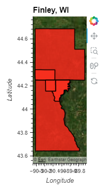
plot = finley_polygons.hvplot(
    geo=True,  # Ensures the plot recognizes geographic data
    title='Finley, WI',  # Confirmed title, adjust as necessary
    tiles='EsriImagery',  # Uses Esri Imagery basemap for background
    color='red',  # Optional: Sets the color of the boundary
    line_width=2,  # Optional: Sets the width of the boundary lines
    alpha=0.8,  # Optional: Sets the transparency of the boundary lines
    figsize=(12, 8)  # Optional: Adjusts the size of the plot
)

# Display the plot
plot

/opt/conda/lib/python3.11/site-packages/pandas/core/frame.py:706: DeprecationWarning: Passing a BlockManager to GeoDataFrame is deprecated and will raise in a future version. Use public APIs instead.
  warnings.warn(
/opt/conda/lib/python3.11/site-packages/geopandas/geodataframe.py:1645: DeprecationWarning: Passing a SingleBlockManager to Series is deprecated and will raise in a future version. Use public APIs instead.
  srs = pd.Series(*args, **kwargs)
WARNING:param.main: hvPlot does not have the concept of a figure, and the figsize keyword will be ignored. The size of each subplot in a layout is set individually using the width and height options.
/opt/conda/lib/python3.11/site-packages/geopandas/geodataframe.py:1645: DeprecationWarning: Passing a SingleBlockManager to Series is deprecated and will raise in a future version. Use public APIs instead.
  srs = pd.Series(*args, **kwargs)
/opt/conda/lib/python3.11/site-packages/geopandas/geodataframe.py:1645: DeprecationWarning: Passing a SingleBlockManager to Series is deprecated and will raise in a future version. Use public APIs instead.
  srs = pd.Series(*args, **kwargs)

The following Python script initializes and uses an object named AppeearsDownloader for downloading MODIS NDVI and EVI data. Here are the main points of the script:

1. Download Specifications: The download_specs list contains dictionaries specifying the data to be downloaded. Each dictionary includes a unique key to identify the download task and a layer specifying the type of data (NDVI or EVI) at a 250-meter resolution with a 16-day frequency.

2. download_data Function: This function is defined to handle the download process for each data type specified in download_specs. It takes a single specs dictionary as an argument, which contains the details needed to configure the downloader.

3. AppeearsDownloader Configuration:
   • download_key: A unique identifier for the download task.
   • ea_dir: The directory where data will be saved, though data_dir is referenced without being previously defined in the provided code.
   • product: Specifies the MODIS product code (MOD13Q1.061), which is common for both NDVI and EVI data.
   • layer: Specifies the particular data layer to download, taken from specs.
   • date Range and Recurring: The data is set to be downloaded for the period from June 1 to June 30, recurring annually from 2020 to 2023.
   • polygon: The geographic area for the data download is specified by finley_polygons, though this variable is also referenced without a prior definition.

4. Error Handling: The script includes a try-except block to handle and report any errors that occur during the download process, ensuring that the script can gracefully handle failures by reporting them.

5. Executing Downloads: The script iterates over each specification in download_specs, calling download_data for both NDVI and EVI data. This loop automates the process of setting up and starting each download task according to the specifications.

This structure ensures that the script is modular and can handle downloading different types of data by simply modifying the download_specs list, making it flexible and reusable for different datasets and time periods.

# Initialize AppeearsDownloader for both MODIS NDVI and EVI data
download_specs = [
    {'key': 'cc-ndvi', 'layer': '_250m_16_days_NDVI'},
    {'key': 'cc-evi', 'layer': '_250m_16_days_EVI'}
]

def download_data(specs):
    try:
        downloader = eaapp.AppeearsDownloader(
            download_key=specs['key'],
            ea_dir=data_dir,
            product='MOD13Q1.061',
            layer=specs['layer'],
            start_date="06-01",
            end_date="06-30",
            recurring=True,
            year_range=[2020, 2023],
            polygon=finley_polygons
        )
        downloader.download_files(cache=True)
    except Exception as e:
        print(f"Failed to download {specs['key']} data due to: {e}")

# Download data for both NDVI and EVI
for spec in download_specs:
    download_data(spec)

/opt/conda/lib/python3.11/site-packages/pandas/core/frame.py:706: DeprecationWarning: Passing a BlockManager to GeoDataFrame is deprecated and will raise in a future version. Use public APIs instead.
  warnings.warn(
/opt/conda/lib/python3.11/site-packages/geopandas/geoseries.py:221: DeprecationWarning: Passing a SingleBlockManager to GeoSeries is deprecated and will raise in a future version. Use public APIs instead.
  super().__init__(data, index=index, name=name, **kwargs)
/opt/conda/lib/python3.11/site-packages/geopandas/geodataframe.py:1645: DeprecationWarning: Passing a SingleBlockManager to Series is deprecated and will raise in a future version. Use public APIs instead.
  srs = pd.Series(*args, **kwargs)
/opt/conda/lib/python3.11/site-packages/pandas/core/frame.py:706: DeprecationWarning: Passing a BlockManager to GeoDataFrame is deprecated and will raise in a future version. Use public APIs instead.
  warnings.warn(
/opt/conda/lib/python3.11/site-packages/pandas/core/frame.py:706: DeprecationWarning: Passing a BlockManager to GeoDataFrame is deprecated and will raise in a future version. Use public APIs instead.
  warnings.warn(
/opt/conda/lib/python3.11/site-packages/geopandas/geodataframe.py:1645: DeprecationWarning: Passing a SingleBlockManager to Series is deprecated and will raise in a future version. Use public APIs instead.
  srs = pd.Series(*args, **kwargs)
/opt/conda/lib/python3.11/site-packages/geopandas/geodataframe.py:1645: DeprecationWarning: Passing a SingleBlockManager to Series is deprecated and will raise in a future version. Use public APIs instead.
  srs = pd.Series(*args, **kwargs)
/opt/conda/lib/python3.11/site-packages/geopandas/geoseries.py:221: DeprecationWarning: Passing a SingleBlockManager to GeoSeries is deprecated and will raise in a future version. Use public APIs instead.
  super().__init__(data, index=index, name=name, **kwargs)
/opt/conda/lib/python3.11/site-packages/pandas/core/frame.py:706: DeprecationWarning: Passing a BlockManager to GeoDataFrame is deprecated and will raise in a future version. Use public APIs instead.
  warnings.warn(
/opt/conda/lib/python3.11/site-packages/geopandas/geoseries.py:221: DeprecationWarning: Passing a SingleBlockManager to GeoSeries is deprecated and will raise in a future version. Use public APIs instead.
  super().__init__(data, index=index, name=name, **kwargs)
/opt/conda/lib/python3.11/site-packages/geopandas/geodataframe.py:1645: DeprecationWarning: Passing a SingleBlockManager to Series is deprecated and will raise in a future version. Use public APIs instead.
  srs = pd.Series(*args, **kwargs)
/opt/conda/lib/python3.11/site-packages/pandas/core/frame.py:706: DeprecationWarning: Passing a BlockManager to GeoDataFrame is deprecated and will raise in a future version. Use public APIs instead.
  warnings.warn(
/opt/conda/lib/python3.11/site-packages/pandas/core/frame.py:706: DeprecationWarning: Passing a BlockManager to GeoDataFrame is deprecated and will raise in a future version. Use public APIs instead.
  warnings.warn(
/opt/conda/lib/python3.11/site-packages/geopandas/geodataframe.py:1645: DeprecationWarning: Passing a SingleBlockManager to Series is deprecated and will raise in a future version. Use public APIs instead.
  srs = pd.Series(*args, **kwargs)
/opt/conda/lib/python3.11/site-packages/geopandas/geodataframe.py:1645: DeprecationWarning: Passing a SingleBlockManager to Series is deprecated and will raise in a future version. Use public APIs instead.
  srs = pd.Series(*args, **kwargs)
/opt/conda/lib/python3.11/site-packages/geopandas/geoseries.py:221: DeprecationWarning: Passing a SingleBlockManager to GeoSeries is deprecated and will raise in a future version. Use public APIs instead.
  super().__init__(data, index=index, name=name, **kwargs)

glob is a function from the glob module in Python’s standard library. It is used to find all the pathnames matching a specified pattern according to the rules used by the Unix shell, although the results are returned in arbitrary order. Files are found by matching patterns with directory paths and file names using wildcard characters.

# Get list of NDVI tif file paths
ndvi_paths = sorted(glob(os.path.join(data_dir, 'cc-ndvi', '*', '*NDVI*.tif')))
# Get list of EVI tif file paths
evi_paths = sorted(glob(os.path.join(data_dir, 'cc-evi', '*', '*EVI*.tif')))

print(f"Number of NDVI files: {len(ndvi_paths)}")
print(f"Number of EVI files: {len(evi_paths)}")

Number of NDVI files: 12
Number of EVI files: 12

ndvi_paths

['/home/jovyan/finley-data/cc-ndvi/MOD13Q1.061_2020138_to_2023181/MOD13Q1.061__250m_16_days_NDVI_doy2020145_aid0001.tif',
 '/home/jovyan/finley-data/cc-ndvi/MOD13Q1.061_2020138_to_2023181/MOD13Q1.061__250m_16_days_NDVI_doy2020161_aid0001.tif',
 '/home/jovyan/finley-data/cc-ndvi/MOD13Q1.061_2020138_to_2023181/MOD13Q1.061__250m_16_days_NDVI_doy2020177_aid0001.tif',
 '/home/jovyan/finley-data/cc-ndvi/MOD13Q1.061_2020138_to_2023181/MOD13Q1.061__250m_16_days_NDVI_doy2021145_aid0001.tif',
 '/home/jovyan/finley-data/cc-ndvi/MOD13Q1.061_2020138_to_2023181/MOD13Q1.061__250m_16_days_NDVI_doy2021161_aid0001.tif',
 '/home/jovyan/finley-data/cc-ndvi/MOD13Q1.061_2020138_to_2023181/MOD13Q1.061__250m_16_days_NDVI_doy2021177_aid0001.tif',
 '/home/jovyan/finley-data/cc-ndvi/MOD13Q1.061_2020138_to_2023181/MOD13Q1.061__250m_16_days_NDVI_doy2022145_aid0001.tif',
 '/home/jovyan/finley-data/cc-ndvi/MOD13Q1.061_2020138_to_2023181/MOD13Q1.061__250m_16_days_NDVI_doy2022161_aid0001.tif',
 '/home/jovyan/finley-data/cc-ndvi/MOD13Q1.061_2020138_to_2023181/MOD13Q1.061__250m_16_days_NDVI_doy2022177_aid0001.tif',
 '/home/jovyan/finley-data/cc-ndvi/MOD13Q1.061_2020138_to_2023181/MOD13Q1.061__250m_16_days_NDVI_doy2023145_aid0001.tif',
 '/home/jovyan/finley-data/cc-ndvi/MOD13Q1.061_2020138_to_2023181/MOD13Q1.061__250m_16_days_NDVI_doy2023161_aid0001.tif',
 '/home/jovyan/finley-data/cc-ndvi/MOD13Q1.061_2020138_to_2023181/MOD13Q1.061__250m_16_days_NDVI_doy2023177_aid0001.tif']

evi_paths

['/home/jovyan/finley-data/cc-evi/MOD13Q1.061_2020138_to_2023181/MOD13Q1.061__250m_16_days_EVI_doy2020145_aid0001.tif',
 '/home/jovyan/finley-data/cc-evi/MOD13Q1.061_2020138_to_2023181/MOD13Q1.061__250m_16_days_EVI_doy2020161_aid0001.tif',
 '/home/jovyan/finley-data/cc-evi/MOD13Q1.061_2020138_to_2023181/MOD13Q1.061__250m_16_days_EVI_doy2020177_aid0001.tif',
 '/home/jovyan/finley-data/cc-evi/MOD13Q1.061_2020138_to_2023181/MOD13Q1.061__250m_16_days_EVI_doy2021145_aid0001.tif',
 '/home/jovyan/finley-data/cc-evi/MOD13Q1.061_2020138_to_2023181/MOD13Q1.061__250m_16_days_EVI_doy2021161_aid0001.tif',
 '/home/jovyan/finley-data/cc-evi/MOD13Q1.061_2020138_to_2023181/MOD13Q1.061__250m_16_days_EVI_doy2021177_aid0001.tif',
 '/home/jovyan/finley-data/cc-evi/MOD13Q1.061_2020138_to_2023181/MOD13Q1.061__250m_16_days_EVI_doy2022145_aid0001.tif',
 '/home/jovyan/finley-data/cc-evi/MOD13Q1.061_2020138_to_2023181/MOD13Q1.061__250m_16_days_EVI_doy2022161_aid0001.tif',
 '/home/jovyan/finley-data/cc-evi/MOD13Q1.061_2020138_to_2023181/MOD13Q1.061__250m_16_days_EVI_doy2022177_aid0001.tif',
 '/home/jovyan/finley-data/cc-evi/MOD13Q1.061_2020138_to_2023181/MOD13Q1.061__250m_16_days_EVI_doy2023145_aid0001.tif',
 '/home/jovyan/finley-data/cc-evi/MOD13Q1.061_2020138_to_2023181/MOD13Q1.061__250m_16_days_EVI_doy2023161_aid0001.tif',
 '/home/jovyan/finley-data/cc-evi/MOD13Q1.061_2020138_to_2023181/MOD13Q1.061__250m_16_days_EVI_doy2023177_aid0001.tif']

• scale_factor: Dividing by scale_factor is essential, confirming the correct approach to transform scaled integer data back to real float values (e.g., dividing by 10000 if scale_factor is based on data description given at https://lpdaac.usgs.gov/products/myd13q1v061/).
• doy_start and doy_end: These parameters are utilized to slice the filename to extract date information. The exact values are based on the naming convention of the files.

This code structure is exemplary for batch processing of geospatial raster data, applying necessary corrections, and organizing it for time-series analysis or other environmental data evaluations.

scale_factor = 10000
doy_start = -19
doy_end = -12

ndvi_das = []
evi_das = []

# Function to open and process TIF files
def process_tif(paths, variable_name, scale_factor, doy_start, doy_end):
    das = []
    for path in paths:
        # Get date from file name
        doy = path[doy_start:doy_end]
        date = pd.to_datetime(doy, format='%Y%j')

        # Open dataset
        da = rxr.open_rasterio(path, masked=True).squeeze()

        # Add date dimension and clean up metadata
        da = da.assign_coords({'date': date})
        da = da.expand_dims({'date': 1})
        da.name = variable_name

        # Multiply by scale factor
        da = da / scale_factor

        # Prepare for concatenation
        das.append(da)
    return das

# Process NDVI and EVI data
ndvi_das = process_tif(ndvi_paths, 'NDVI', scale_factor, doy_start, doy_end)
evi_das = process_tif(evi_paths, 'EVI', scale_factor, doy_start, doy_end)

# Print the number of processed files
print(f"Processed NDVI datasets: {len(ndvi_das)}")
print(f"Processed EVI datasets: {len(evi_das)}")

Processed NDVI datasets: 12
Processed EVI datasets: 12

# Combine NDVI data arrays across different dates into a single DataArray
# 'ndvi_das' is a list of xarray DataArray objects, each representing NDVI data for different dates
# 'coords' specifies the coordinate along which to align and combine the data arrays

ndvi_da = xr.combine_by_coords(ndvi_das, coords=['date'])
ndvi_da

# The resulting 'ndvi_da' is an xarray DataArray that merges all the NDVI datasets into one,
# indexed by the 'date' coordinate which allows for easier manipulation and analysis over time

<xarray.Dataset>
Dimensions:      (x: 286, y: 502, date: 12)
Coordinates:
    band         int64 1
  * x            (x) float64 -90.32 -90.32 -90.31 ... -89.73 -89.73 -89.72
  * y            (y) float64 44.68 44.68 44.68 44.68 ... 43.65 43.64 43.64 43.64
    spatial_ref  int64 0
  * date         (date) datetime64[ns] 2020-05-24 2020-06-09 ... 2023-06-26
Data variables:
    NDVI         (date, y, x) float32 0.7044 0.7176 0.6629 ... 0.555 0.555

xarray.Dataset

• Dimensions:
  • x: 286
  • y: 502
  • date: 12
• Coordinates: (5)
  • band
    ()
    int64
    1

    array(1)

  • x
    (x)
    float64
    -90.32 -90.32 ... -89.73 -89.72

    array([-90.317708, -90.315625, -90.313542, ..., -89.728125, -89.726042,
           -89.723958])

  • y
    (y)
    float64
    44.68 44.68 44.68 ... 43.64 43.64

    array([44.684375, 44.682292, 44.680208, ..., 43.644792, 43.642708, 43.640625])

  • spatial_ref
    ()
    int64
    0

    crs_wkt :

    GEOGCS["WGS 84",DATUM["WGS_1984",SPHEROID["WGS 84",6378137,298.257223563,AUTHORITY["EPSG","7030"]],AUTHORITY["EPSG","6326"]],PRIMEM["Greenwich",0,AUTHORITY["EPSG","8901"]],UNIT["degree",0.0174532925199433,AUTHORITY["EPSG","9122"]],AXIS["Latitude",NORTH],AXIS["Longitude",EAST],AUTHORITY["EPSG","4326"]]

    semi_major_axis :

    6378137.0

    semi_minor_axis :

    6356752.314245179

    inverse_flattening :

    298.257223563

    reference_ellipsoid_name :

    WGS 84

    longitude_of_prime_meridian :

    0.0

    prime_meridian_name :

    Greenwich

    geographic_crs_name :

    WGS 84

    horizontal_datum_name :

    World Geodetic System 1984

    grid_mapping_name :

    latitude_longitude

    spatial_ref :

    GEOGCS["WGS 84",DATUM["WGS_1984",SPHEROID["WGS 84",6378137,298.257223563,AUTHORITY["EPSG","7030"]],AUTHORITY["EPSG","6326"]],PRIMEM["Greenwich",0,AUTHORITY["EPSG","8901"]],UNIT["degree",0.0174532925199433,AUTHORITY["EPSG","9122"]],AXIS["Latitude",NORTH],AXIS["Longitude",EAST],AUTHORITY["EPSG","4326"]]

    GeoTransform :

    -90.31874999160073 0.002083333333139592 0.0 44.68541666251111 0.0 -0.002083333333139592

    array(0)

  • date
    (date)
    datetime64[ns]
    2020-05-24 ... 2023-06-26

    array(['2020-05-24T00:00:00.000000000', '2020-06-09T00:00:00.000000000',
           '2020-06-25T00:00:00.000000000', '2021-05-25T00:00:00.000000000',
           '2021-06-10T00:00:00.000000000', '2021-06-26T00:00:00.000000000',
           '2022-05-25T00:00:00.000000000', '2022-06-10T00:00:00.000000000',
           '2022-06-26T00:00:00.000000000', '2023-05-25T00:00:00.000000000',
           '2023-06-10T00:00:00.000000000', '2023-06-26T00:00:00.000000000'],
          dtype='datetime64[ns]')

• Data variables: (1)
  • NDVI
    (date, y, x)
    float32
    0.7044 0.7176 ... 0.555 0.555

    array([[[0.7044, 0.7176, 0.6629, ..., 0.7867, 0.5898, 0.6046],
            [0.8609, 0.8311, 0.7319, ..., 0.571 , 0.5708, 0.5898],
            [0.8648, 0.8675, 0.8675, ..., 0.5801, 0.5272, 0.5738],
            ...,
            [0.8015, 0.7137, 0.6496, ..., 0.7907, 0.7961, 0.7961],
            [0.7216, 0.8727, 0.737 , ..., 0.7006, 0.7563, 0.7563],
            [0.8645, 0.8727, 0.8727, ..., 0.6799, 0.6754, 0.6754]],
    
           [[0.5064, 0.6056, 0.5743, ..., 0.7275, 0.6965, 0.7043],
            [0.8655, 0.8604, 0.7112, ..., 0.5393, 0.6762, 0.7043],
            [0.8634, 0.8583, 0.8583, ..., 0.4209, 0.6207, 0.6183],
            ...,
            [0.8292, 0.807 , 0.7433, ..., 0.8241, 0.8528, 0.8528],
            [0.7296, 0.8569, 0.8607, ..., 0.651 , 0.6938, 0.6938],
            [0.9097, 0.7918, 0.7918, ..., 0.7014, 0.7146, 0.7146]],
    
           [[0.8791, 0.7364, 0.7302, ..., 0.8169, 0.7678, 0.7963],
            [0.8779, 0.8569, 0.7968, ..., 0.6994, 0.735 , 0.7847],
            [0.8817, 0.8602, 0.8602, ..., 0.6989, 0.735 , 0.7189],
            ...,
    ...
            [0.7218, 0.6682, 0.5519, ..., 0.7774, 0.8013, 0.8013],
            [0.7212, 0.7867, 0.7786, ..., 0.7156, 0.8013, 0.8013],
            [0.8566, 0.8452, 0.8452, ..., 0.7156, 0.7099, 0.7099]],
    
           [[0.5625, 0.6023, 0.6243, ..., 0.7433, 0.8359, 0.7003],
            [0.7829, 0.6676, 0.7247, ..., 0.5339, 0.7433, 0.7254],
            [0.86  , 0.7902, 0.7902, ..., 0.4011, 0.7015, 0.6787],
            ...,
            [0.7742, 0.6993, 0.6949, ..., 0.8166, 0.8042, 0.8042],
            [0.8401, 0.8457, 0.8379, ..., 0.5927, 0.5743, 0.5743],
            [0.8464, 0.8457, 0.8457, ..., 0.6184, 0.534 , 0.534 ]],
    
           [[0.821 , 0.8536, 0.777 , ..., 0.691 , 0.7793, 0.7642],
            [0.8643, 0.8519, 0.777 , ..., 0.7305, 0.7374, 0.7831],
            [0.8844, 0.8519, 0.8519, ..., 0.3946, 0.65  , 0.6944],
            ...,
            [0.8512, 0.8039, 0.7498, ..., 0.6853, 0.7597, 0.7597],
            [0.9152, 0.8039, 0.8238, ..., 0.555 , 0.4974, 0.4974],
            [0.9096, 0.9152, 0.9152, ..., 0.5908, 0.555 , 0.555 ]]],
          dtype=float32)

• Indexes: (3)
  • x
    PandasIndex

    PandasIndex(Index([-90.31770832493416, -90.31562499160103, -90.31354165826788,
           -90.31145832493473,  -90.3093749916016, -90.30729165826847,
           -90.30520832493532, -90.30312499160217, -90.30104165826904,
           -90.29895832493591,
           ...
           -89.74270832498763,  -89.7406249916545, -89.73854165832135,
            -89.7364583249882, -89.73437499165507, -89.73229165832194,
            -89.7302083249888, -89.72812499165565, -89.72604165832252,
           -89.72395832498938],
          dtype='float64', name='x', length=286))

  • y
    PandasIndex

    PandasIndex(Index([44.684374995844536, 44.682291662511396,  44.68020832917826,
            44.67812499584512,  44.67604166251198,  44.67395832917884,
             44.6718749958457,  44.66979166251256,  44.66770832917942,
            44.66562499584628,
           ...
            43.65937499593986,  43.65729166260672,  43.65520832927358,
            43.65312499594044,   43.6510416626073,  43.64895832927416,
            43.64687499594102,  43.64479166260788,  43.64270832927474,
             43.6406249959416],
          dtype='float64', name='y', length=502))

  • date
    PandasIndex

    PandasIndex(DatetimeIndex(['2020-05-24', '2020-06-09', '2020-06-25', '2021-05-25',
                   '2021-06-10', '2021-06-26', '2022-05-25', '2022-06-10',
                   '2022-06-26', '2023-05-25', '2023-06-10', '2023-06-26'],
                  dtype='datetime64[ns]', name='date', freq=None))

• Attributes: (0)

evi_da = xr.combine_by_coords(evi_das, coords=['date'])
evi_da

<xarray.Dataset>
Dimensions:      (x: 286, y: 502, date: 12)
Coordinates:
    band         int64 1
  * x            (x) float64 -90.32 -90.32 -90.31 ... -89.73 -89.73 -89.72
  * y            (y) float64 44.68 44.68 44.68 44.68 ... 43.65 43.64 43.64 43.64
    spatial_ref  int64 0
  * date         (date) datetime64[ns] 2020-05-24 2020-06-09 ... 2023-06-26
Data variables:
    EVI          (date, y, x) float32 0.5624 0.5019 0.5187 ... 0.3659 0.3659

xarray.Dataset

• Dimensions:
  • x: 286
  • y: 502
  • date: 12
• Coordinates: (5)
  • band
    ()
    int64
    1

    array(1)

  • x
    (x)
    float64
    -90.32 -90.32 ... -89.73 -89.72

    array([-90.317708, -90.315625, -90.313542, ..., -89.728125, -89.726042,
           -89.723958])

  • y
    (y)
    float64
    44.68 44.68 44.68 ... 43.64 43.64

    array([44.684375, 44.682292, 44.680208, ..., 43.644792, 43.642708, 43.640625])

  • spatial_ref
    ()
    int64
    0

    crs_wkt :

    GEOGCS["WGS 84",DATUM["WGS_1984",SPHEROID["WGS 84",6378137,298.257223563,AUTHORITY["EPSG","7030"]],AUTHORITY["EPSG","6326"]],PRIMEM["Greenwich",0,AUTHORITY["EPSG","8901"]],UNIT["degree",0.0174532925199433,AUTHORITY["EPSG","9122"]],AXIS["Latitude",NORTH],AXIS["Longitude",EAST],AUTHORITY["EPSG","4326"]]

    semi_major_axis :

    6378137.0

    semi_minor_axis :

    6356752.314245179

    inverse_flattening :

    298.257223563

    reference_ellipsoid_name :

    WGS 84

    longitude_of_prime_meridian :

    0.0

    prime_meridian_name :

    Greenwich

    geographic_crs_name :

    WGS 84

    horizontal_datum_name :

    World Geodetic System 1984

    grid_mapping_name :

    latitude_longitude

    spatial_ref :

    GEOGCS["WGS 84",DATUM["WGS_1984",SPHEROID["WGS 84",6378137,298.257223563,AUTHORITY["EPSG","7030"]],AUTHORITY["EPSG","6326"]],PRIMEM["Greenwich",0,AUTHORITY["EPSG","8901"]],UNIT["degree",0.0174532925199433,AUTHORITY["EPSG","9122"]],AXIS["Latitude",NORTH],AXIS["Longitude",EAST],AUTHORITY["EPSG","4326"]]

    GeoTransform :

    -90.31874999160073 0.002083333333139592 0.0 44.68541666251111 0.0 -0.002083333333139592

    array(0)

  • date
    (date)
    datetime64[ns]
    2020-05-24 ... 2023-06-26

    array(['2020-05-24T00:00:00.000000000', '2020-06-09T00:00:00.000000000',
           '2020-06-25T00:00:00.000000000', '2021-05-25T00:00:00.000000000',
           '2021-06-10T00:00:00.000000000', '2021-06-26T00:00:00.000000000',
           '2022-05-25T00:00:00.000000000', '2022-06-10T00:00:00.000000000',
           '2022-06-26T00:00:00.000000000', '2023-05-25T00:00:00.000000000',
           '2023-06-10T00:00:00.000000000', '2023-06-26T00:00:00.000000000'],
          dtype='datetime64[ns]')

• Data variables: (1)
  • EVI
    (date, y, x)
    float32
    0.5624 0.5019 ... 0.3659 0.3659

    array([[[0.5624, 0.5019, 0.5187, ..., 0.5289, 0.2924, 0.346 ],
            [0.5961, 0.627 , 0.4578, ..., 0.2528, 0.2611, 0.2893],
            [0.6083, 0.6174, 0.6174, ..., 0.1392, 0.2427, 0.3166],
            ...,
            [0.626 , 0.5192, 0.4656, ..., 0.4804, 0.5178, 0.5178],
            [0.5672, 0.6801, 0.5994, ..., 0.4127, 0.49  , 0.49  ],
            [0.7198, 0.6458, 0.6458, ..., 0.4017, 0.4979, 0.4979]],
    
           [[0.3294, 0.4317, 0.4281, ..., 0.4483, 0.385 , 0.4475],
            [0.6558, 0.6897, 0.5292, ..., 0.1353, 0.3108, 0.4713],
            [0.6767, 0.6584, 0.6584, ..., 0.067 , 0.2016, 0.3555],
            ...,
            [0.6413, 0.6308, 0.571 , ..., 0.603 , 0.6622, 0.6622],
            [0.5529, 0.7014, 0.6535, ..., 0.4285, 0.4638, 0.4638],
            [0.7216, 0.5769, 0.5769, ..., 0.4632, 0.5325, 0.5325]],
    
           [[0.7103, 0.4844, 0.5009, ..., 0.4407, 0.3944, 0.4678],
            [0.6807, 0.6431, 0.5621, ..., 0.2644, 0.3817, 0.5401],
            [0.6986, 0.644 , 0.644 , ..., 0.196 , 0.3817, 0.3232],
            ...,
    ...
            [0.585 , 0.5267, 0.4146, ..., 0.4875, 0.5239, 0.5239],
            [0.5531, 0.6659, 0.6684, ..., 0.4054, 0.5239, 0.5239],
            [0.7151, 0.7041, 0.7041, ..., 0.3972, 0.4409, 0.4409]],
    
           [[0.3913, 0.4285, 0.4517, ..., 0.4107, 0.5671, 0.4197],
            [0.5606, 0.4488, 0.5121, ..., 0.1538, 0.424 , 0.4097],
            [0.6782, 0.5792, 0.5792, ..., 0.0807, 0.3555, 0.3813],
            ...,
            [0.6177, 0.5109, 0.5272, ..., 0.5897, 0.6075, 0.6075],
            [0.7182, 0.7137, 0.7094, ..., 0.3504, 0.3452, 0.3452],
            [0.7601, 0.7513, 0.7513, ..., 0.3796, 0.3562, 0.3562]],
    
           [[0.6155, 0.6445, 0.5434, ..., 0.3527, 0.496 , 0.4993],
            [0.665 , 0.6262, 0.5167, ..., 0.3566, 0.393 , 0.4978],
            [0.6808, 0.6288, 0.6288, ..., 0.0929, 0.2437, 0.3523],
            ...,
            [0.6355, 0.5653, 0.5261, ..., 0.4688, 0.5983, 0.5983],
            [0.7175, 0.5653, 0.5815, ..., 0.3434, 0.3039, 0.3039],
            [0.6761, 0.6851, 0.6851, ..., 0.3741, 0.3659, 0.3659]]],
          dtype=float32)

• Indexes: (3)
  • x
    PandasIndex

    PandasIndex(Index([-90.31770832493416, -90.31562499160103, -90.31354165826788,
           -90.31145832493473,  -90.3093749916016, -90.30729165826847,
           -90.30520832493532, -90.30312499160217, -90.30104165826904,
           -90.29895832493591,
           ...
           -89.74270832498763,  -89.7406249916545, -89.73854165832135,
            -89.7364583249882, -89.73437499165507, -89.73229165832194,
            -89.7302083249888, -89.72812499165565, -89.72604165832252,
           -89.72395832498938],
          dtype='float64', name='x', length=286))

  • y
    PandasIndex

    PandasIndex(Index([44.684374995844536, 44.682291662511396,  44.68020832917826,
            44.67812499584512,  44.67604166251198,  44.67395832917884,
             44.6718749958457,  44.66979166251256,  44.66770832917942,
            44.66562499584628,
           ...
            43.65937499593986,  43.65729166260672,  43.65520832927358,
            43.65312499594044,   43.6510416626073,  43.64895832927416,
            43.64687499594102,  43.64479166260788,  43.64270832927474,
             43.6406249959416],
          dtype='float64', name='y', length=502))

  • date
    PandasIndex

    PandasIndex(DatetimeIndex(['2020-05-24', '2020-06-09', '2020-06-25', '2021-05-25',
                   '2021-06-10', '2021-06-26', '2022-05-25', '2022-06-10',
                   '2022-06-26', '2023-05-25', '2023-06-10', '2023-06-26'],
                  dtype='datetime64[ns]', name='date', freq=None))

• Attributes: (0)

### Part 2: Comparative Analysis of NDVI and EVI

Objective:This part explores the comparison of the sensitivity and responsiveness of NDVI and EVI to different vegetation types or stress conditions. It uses NDVI and EVI data to determine how each index responds under various environmental conditions. This analysis can help in understanding which index is better suited for specific applications or ecosystems.

# 'ndvi_da' and 'evi_da' are your datasets
# Function to plot data for a given year
def plot_data_by_year(da, variable_name, year, polygons):
    # Select data for specified year
    data_slice = da.sel(date=str(year))

    # Mean over all dates within the year to get an average image
    mean_data = data_slice.mean('date')
    
    # Extract the data for the specific variable
    data_variable = mean_data[variable_name]
    
    # Create the plot
    image_plot = data_variable.hvplot(x='x', y='y', cmap='PiYG', geo=True, width=300, height=300, title=f'{variable_name} {year}')
    polygon_plot = polygons.hvplot(geo=True, fill_color=None, line_color='black', width=300, height=300)
    
    # Overlay the plots
    return image_plot * polygon_plot

# Years to plot
years = [2020, 2021, 2022, 2023]

# Collect plots for NDVI and EVI separately
ndvi_plots = [plot_data_by_year(ndvi_da, 'NDVI', year, finley_polygons) for year in years]
evi_plots = [plot_data_by_year(evi_da, 'EVI', year, finley_polygons) for year in years]

# Combine plots into rows
ndvi_row = hv.Layout(ndvi_plots).cols(len(years))  # NDVI plots in one row
evi_row = hv.Layout(evi_plots).cols(len(years))   # EVI plots in one row

# Combine the two rows into a final layout
final_plot = ndvi_row + evi_row

# Display the final plot
final_plot

/opt/conda/lib/python3.11/site-packages/geopandas/geodataframe.py:1645: DeprecationWarning: Passing a SingleBlockManager to Series is deprecated and will raise in a future version. Use public APIs instead.
  srs = pd.Series(*args, **kwargs)
/opt/conda/lib/python3.11/site-packages/geopandas/geodataframe.py:1645: DeprecationWarning: Passing a SingleBlockManager to Series is deprecated and will raise in a future version. Use public APIs instead.
  srs = pd.Series(*args, **kwargs)
/opt/conda/lib/python3.11/site-packages/geopandas/geodataframe.py:1645: DeprecationWarning: Passing a SingleBlockManager to Series is deprecated and will raise in a future version. Use public APIs instead.
  srs = pd.Series(*args, **kwargs)
/opt/conda/lib/python3.11/site-packages/geopandas/geodataframe.py:1645: DeprecationWarning: Passing a SingleBlockManager to Series is deprecated and will raise in a future version. Use public APIs instead.
  srs = pd.Series(*args, **kwargs)
/opt/conda/lib/python3.11/site-packages/geopandas/geodataframe.py:1645: DeprecationWarning: Passing a SingleBlockManager to Series is deprecated and will raise in a future version. Use public APIs instead.
  srs = pd.Series(*args, **kwargs)
/opt/conda/lib/python3.11/site-packages/geopandas/geodataframe.py:1645: DeprecationWarning: Passing a SingleBlockManager to Series is deprecated and will raise in a future version. Use public APIs instead.
  srs = pd.Series(*args, **kwargs)
/opt/conda/lib/python3.11/site-packages/geopandas/geodataframe.py:1645: DeprecationWarning: Passing a SingleBlockManager to Series is deprecated and will raise in a future version. Use public APIs instead.
  srs = pd.Series(*args, **kwargs)
/opt/conda/lib/python3.11/site-packages/geopandas/geodataframe.py:1645: DeprecationWarning: Passing a SingleBlockManager to Series is deprecated and will raise in a future version. Use public APIs instead.
  srs = pd.Series(*args, **kwargs)

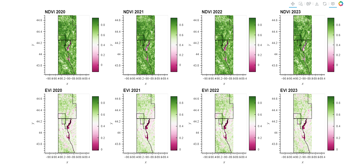
## Observation 👀🔍

The series of NDVI and EVI maps for Finley, Wisconsin, from 2020 to 2023 provide a clear view of the vegetation and hydrological features of the region. These images illustrate the annual dynamics of vegetation health surrounding a central river, which consistently shows lower NDVI and EVI values, indicating minimal or non-existent vegetation.

Spatial and Annual Distribution - Vegetation and Water Body Trends

• River Representation: Throughout the four years, the river consistently exhibits lower values in both NDVI and EVI, confirming its non-vegetative nature. This consistency is an excellent validation of the indices’ effectiveness in differentiating between vegetative areas and water bodies.
• Vegetation Health: Surrounding vegetated areas, likely including riparian zones, show significant greening across the images, indicating healthy or dense vegetation, benefiting from the proximity to water.

Yearly Observations and Detailed Interpretation

• NDVI (2020-2023): The NDVI images display robust vegetation, with noticeable changes over the years that might reflect agricultural cycles, natural vegetation growth, or environmental management practices.
• EVI (2020-2023): EVI maps provide a more nuanced view, highlighting finer vegetation health details, especially in densely vegetated or cultivated areas. EVI’s sensitivity to chlorophyll enhances its ability to depict actual vegetation condition better than NDVI, particularly in high biomass areas.

Key Comparisons: EVI vs. NDVI

• EVI’s Advantages: Compared to NDVI, EVI is less prone to saturation in high vegetation areas, allowing for a clearer differentiation of vegetation health levels. This feature makes EVI particularly valuable for detailed ecological assessments and agricultural management.
• Temporal Vegetation Changes: Variations in color intensity and coverage over the years may suggest significant ecological or climatic events affecting vegetation, such as seasonal variations, agricultural practices changes, or environmental conservation efforts.

These data from NDVI and EVI maps are crucial for understanding the ecological dynamics of Finley, Wisconsin. They support effective environmental and agricultural planning by providing a reliable measure of vegetation health and changes over time. The consistent low values of NDVI and EVI over the river across all years reinforce the indices’ reliability, while the detailed annual changes in surrounding vegetative areas highlight the importance of ongoing monitoring for sustainable management and planning practices. This analysis underscores the value of NDVI and EVI data in environmental management, offering essential insights for stakeholders involved in agriculture, conservation, and urban planning around significant water bodies.

### Part 3: Trend Analysis Over Time

Objective:This part examines how to identify changes in vegetation cover over the time period. It involves calculating the mean NDVI and EVI values and plotting these over time. The goal is to observe trends, such as increasing or decreasing vegetation health, which might indicate environmental changes, the impact of land management policies, or the effects of climatic events like droughts or floods.

#First Code Block

# Calculate yearly means for NDVI and EVI
# Assuming `ndvi_da` and `evi_da` are xarray.DataArrays with a 'date' coordinate.
# Ensure that you're selecting only the data variable if dealing with a Dataset.
if isinstance(ndvi_da, xr.Dataset):
    ndvi_yearly_mean = ndvi_da['NDVI'].groupby('date.year').mean()
    evi_yearly_mean = evi_da['EVI'].groupby('date.year').mean()
else:
    ndvi_yearly_mean = ndvi_da.groupby('date.year').mean()
    evi_yearly_mean = evi_da.groupby('date.year').mean()

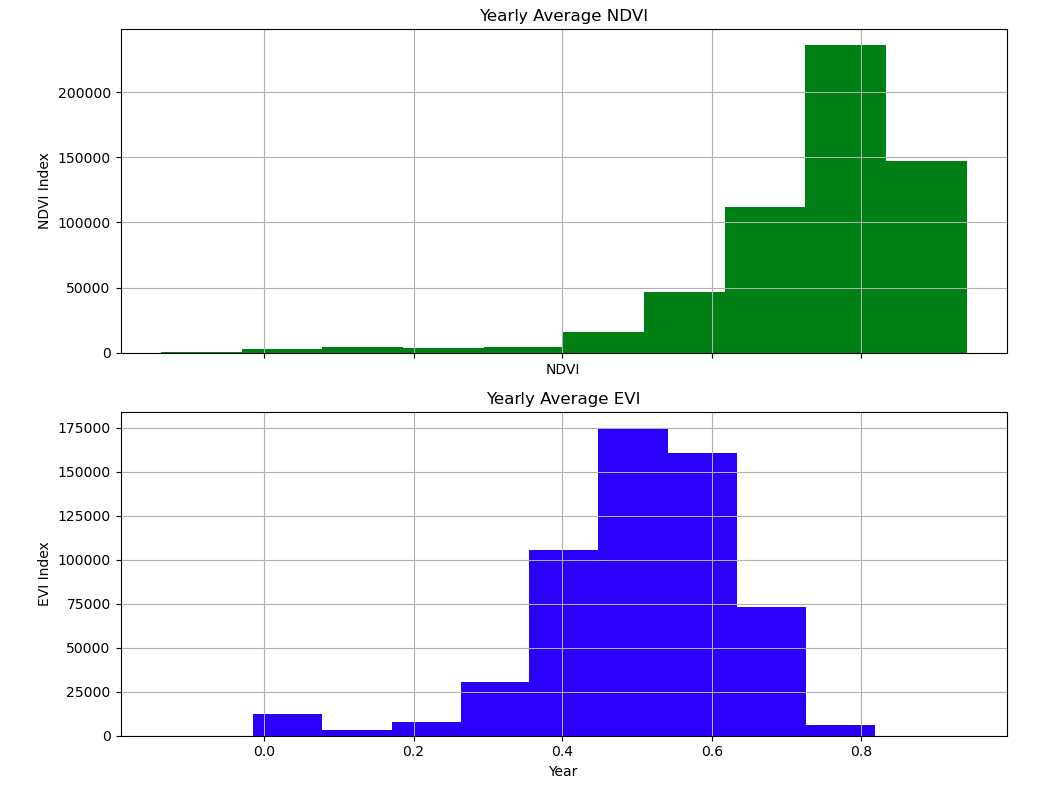
# Plotting the trends over time
fig, axes = plt.subplots(2, 1, figsize=(10, 8), sharex=True)

ndvi_yearly_mean.plot(ax=axes[0], color='green')
axes[0].set_title('Yearly Average NDVI')
axes[0].set_ylabel('NDVI Index')
axes[0].grid(True)

evi_yearly_mean.plot(ax=axes[1], color='blue')
axes[1].set_title('Yearly Average EVI')
axes[1].set_ylabel('EVI Index')
axes[1].grid(True)

plt.xlabel('Year')
plt.tight_layout()
plt.show()

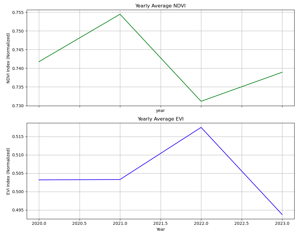
#Second Code Block

# ndvi_da and evi_da are datasets
# Normalize the data if necessary
ndvi_normalized = ndvi_da.mean(dim=['x', 'y'])  # Adjust dimensions if different
evi_normalized = evi_da.mean(dim=['x', 'y'])  # Adjust dimensions if different

# Calculate yearly means
ndvi_yearly_mean = ndvi_normalized.groupby('date.year').mean()
evi_yearly_mean = evi_normalized.groupby('date.year').mean()

# Plotting the trends over time
fig, axes = plt.subplots(2, 1, figsize=(10, 8), sharex=True)

# Make sure to select the correct variable if it's a dataset. Adjust 'variable_name' accordingly.
if isinstance(ndvi_yearly_mean, xr.Dataset):
    ndvi_yearly_mean['NDVI'].plot(ax=axes[0], color='green')  # Replace 'NDVI' with your variable name
else:
    ndvi_yearly_mean.plot(ax=axes[0], color='green')

axes[0].set_title('Yearly Average NDVI')
axes[0].set_ylabel('NDVI Index (Normalized)')
axes[0].grid(True)

if isinstance(evi_yearly_mean, xr.Dataset):
    evi_yearly_mean['EVI'].plot(ax=axes[1], color='blue')  # Replace 'EVI' with your variable name
else:
    evi_yearly_mean.plot(ax=axes[1], color='blue')

axes[1].set_title('Yearly Average EVI')
axes[1].set_ylabel('EVI Index (Normalized)')
axes[1].grid(True)

plt.xlabel('Year')
plt.tight_layout()
plt.show()

💡Point to Note

💡Strategic Approaches to NDVI and EVI Trend Analysis with enhanced Data Handling techniques

Comparison of Code Blocks for NDVI and EVI Mean Processing

First Code Block This block directly checks if the input data (ndvi_da and evi_da) are xarray.Dataset or xarray.DataArray objects and then processes the data accordingly. Here’s a breakdown:

• Dataset vs DataArray: The code uses an isinstance check to determine the type of the data and selects the relevant variable ('NDVI', 'EVI') if it’s a Dataset. This approach is robust when handling data structures that might vary (either single variable data arrays or multi-variable datasets).
• Yearly Averages: It computes the yearly average directly on the data grouped by year, which presumes that the data is pre-scaled or does not require normalization over spatial dimensions (x, y).
• Plotting: Each variable is plotted directly as yearly averages, and the plots are standardized for presentation, not handling any normalization across spatial dimensions in the plotting code itself.

This code is straightforward and assumes that the data is relatively prepared (e.g., spatial averaging is not required or already handled).

Second Code Block

This code takes a different approach, especially in handling the spatial dimensions of the data:

• Normalization: Before computing the yearly means, it averages the data across spatial dimensions (x, y). This step is crucial if the data represents summed values across these dimensions and you want to convert these into mean values to prevent artificially high index values.
• Handling Data Structure: Like the first block, it checks for data types (Dataset vs DataArray) but does this check after normalizing over spatial dimensions and again when plotting. This is more detailed and ensures that no matter where the data structure might vary, it handles it appropriately.
• Plotting: It handles potential datasets after spatial normalization, checking again before plotting, ensuring that even after operations that might change the data structure, the correct plotting method is used.

This approach is more comprehensive in terms of preprocessing, especially useful when the raw data includes extensive spatial information that needs to be simplified into a more manageable form (like mean values per pixel).

Key Improvements and Differences

1. Spatial Normalization: The second block includes an essential step of normalizing across spatial dimensions (x, y), which is critical if your data is structured such that each entry in ndvi_da or evi_da represents an aggregate over a spatial area, rather than an average.

2. Robustness in Data Handling: The second block ensures that at each step where data manipulation might alter the structure (from DataArray to Dataset), the code checks and handles these changes. This makes the code more robust against different data structures that might be passed into it.

3. Plotting Flexibility: Both blocks handle the plotting similarly by ensuring the use of the correct data variable. However, the second block adds checks post any data manipulation, making it flexible to handle changes due to prior computations.

Decision ?

The choice between these two depends on your specific data setup and what preprocessing steps are necessary. If your data is already spatially averaged or if spatial averaging isn’t required, the first code block is simpler and more direct. If your data requires spatial averaging to correctly represent the indices (like NDVI, EVI), the second block provides a more detailed and thorough approach, ensuring the data is appropriately processed for meaningful analysis and visualization.

### Part 4: Change Detection Analysis and Anomaly Detection

Objective:This part investigates how to identify specific areas within Finley that have undergone significant changes in vegetation over a four-year period. It involves calculating the difference in NDVI and EVI values between the first year (2020) and the last year (2023) to map out areas of significant increase or decrease in vegetation health. This analysis can help identify recovery or degradation hotspots.

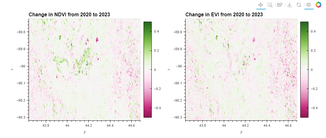
#First block of code
 
# Assume 'ndvi_da' and 'evi_da' are xarray.Dataset objects that might have multiple variables
# Calculate the change in NDVI and EVI over the period
# Make sure to replace 'NDVI' and 'EVI' with the actual variable names if different
ndvi_change = (ndvi_da['NDVI'].sel(date='2023').mean('date') - 
               ndvi_da['NDVI'].sel(date='2020').mean('date'))
evi_change = (evi_da['EVI'].sel(date='2023').mean('date') - 
              evi_da['EVI'].sel(date='2020').mean('date'))

# Interactive plotting using hvplot
ndvi_plot = ndvi_change.hvplot.image(cmap='PiYG', clim=(-0.5, 0.5), width=500, height=400, colorbar=True, title='Change in NDVI from 2020 to 2023')
evi_plot = evi_change.hvplot.image(cmap='PiYG', clim=(-0.5, 0.5), width=500, height=400, colorbar=True, title='Change in EVI from 2020 to 2023')

# Display the plots
ndvi_plot + evi_plot

# Reproducing error 

# Assume 'ndvi_da' and 'evi_da' are xarray.Dataset objects that might have multiple variables
# Calculate the change in NDVI and EVI over the period
# Make sure to replace 'NDVI' and 'EVI' with the actual variable names if different
ndvi_change = (ndvi_da['NDVI'].sel(date='2023').mean('date') - 
               ndvi_da['NDVI'].sel(date='2020').mean('date'))
evi_change = (evi_da['EVI'].sel(date='2023').mean('date') - 
              evi_da['EVI'].sel(date='2020').mean('date'))

# Interactive plotting using hvplot
ndvi_plot = ndvi_change.hvplot.image(x='longitude', y='latitude', cmap='PiYG', clim=(-0.5, 0.5), width=500, height=400, colorbar=True, title='Change in NDVI from 2020 to 2023')
evi_plot = evi_change.hvplot.image(x='longitude', y='latitude', cmap='PiYG', clim=(-0.5, 0.5), width=500, height=400, colorbar=True, title='Change in EVI from 2020 to 2023')

# Display the plots
ndvi_plot + evi_plot

---------------------------------------------------------------------------

DataError                                 Traceback (most recent call last)

Cell In[26], line 13
      9 evi_change = (evi_da['EVI'].sel(date='2023').mean('date') - 
     10               evi_da['EVI'].sel(date='2020').mean('date'))
     12 # Interactive plotting using hvplot
---> 13 ndvi_plot = ndvi_change.hvplot.image(x='longitude', y='latitude', cmap='PiYG', clim=(-0.5, 0.5), width=500, height=400, colorbar=True, title='Change in NDVI from 2020 to 2023')
     14 evi_plot = evi_change.hvplot.image(x='longitude', y='latitude', cmap='PiYG', clim=(-0.5, 0.5), width=500, height=400, colorbar=True, title='Change in EVI from 2020 to 2023')
     16 # Display the plots


File /opt/conda/lib/python3.11/site-packages/hvplot/plotting/core.py:2069, in hvPlot.image(self, x, y, z, colorbar, **kwds)
   2017 def image(self, x=None, y=None, z=None, colorbar=True, **kwds):
   2018     """
   2019     Image plot
   2020 
   (...)
   2067     - Plotly: https://plotly.com/python/imshow/
   2068     """
-> 2069     return self(x, y, z=z, kind="image", colorbar=colorbar, **kwds)


File /opt/conda/lib/python3.11/site-packages/hvplot/plotting/core.py:96, in hvPlotBase.__call__(self, x, y, kind, **kwds)
     93         plot = self._get_converter(x, y, kind, **kwds)(kind, x, y)
     94         return pn.panel(plot, **panel_dict)
---> 96 return self._get_converter(x, y, kind, **kwds)(kind, x, y)


File /opt/conda/lib/python3.11/site-packages/hvplot/converter.py:1267, in HoloViewsConverter.__call__(self, kind, x, y)
   1265     else:
   1266         name = data.name or self.label or self.value_label
-> 1267         dataset = Dataset(data, self.indexes, name)
   1268 else:
   1269     try:


File /opt/conda/lib/python3.11/site-packages/holoviews/core/data/__init__.py:329, in Dataset.__init__(self, data, kdims, vdims, **kwargs)
    326 kdims, vdims = kwargs.get('kdims'), kwargs.get('vdims')
    328 validate_vdims = kwargs.pop('_validate_vdims', True)
--> 329 initialized = Interface.initialize(type(self), data, kdims, vdims,
    330                                    datatype=kwargs.get('datatype'))
    331 (data, self.interface, dims, extra_kws) = initialized
    332 super().__init__(data, **dict(kwargs, **dict(dims, **extra_kws)))


File /opt/conda/lib/python3.11/site-packages/holoviews/core/data/interface.py:253, in Interface.initialize(cls, eltype, data, kdims, vdims, datatype)
    251     continue
    252 try:
--> 253     (data, dims, extra_kws) = interface.init(eltype, data, kdims, vdims)
    254     break
    255 except DataError:


File /opt/conda/lib/python3.11/site-packages/holoviews/core/data/xarray.py:215, in XArrayInterface.init(cls, eltype, data, kdims, vdims)
    213     raise TypeError('Data must be be an xarray Dataset type.')
    214 elif not_found:
--> 215     raise DataError("xarray Dataset must define coordinates "
    216                     "for all defined kdims, %s coordinates not found."
    217                     % not_found, cls)
    219 for vdim in vdims:
    220     if packed:


DataError: xarray Dataset must define coordinates for all defined kdims, [Dimension('longitude'), Dimension('latitude')] coordinates not found.

XArrayInterface expects gridded data, for more information on supported datatypes see http://holoviews.org/user_guide/Gridded_Datasets.html

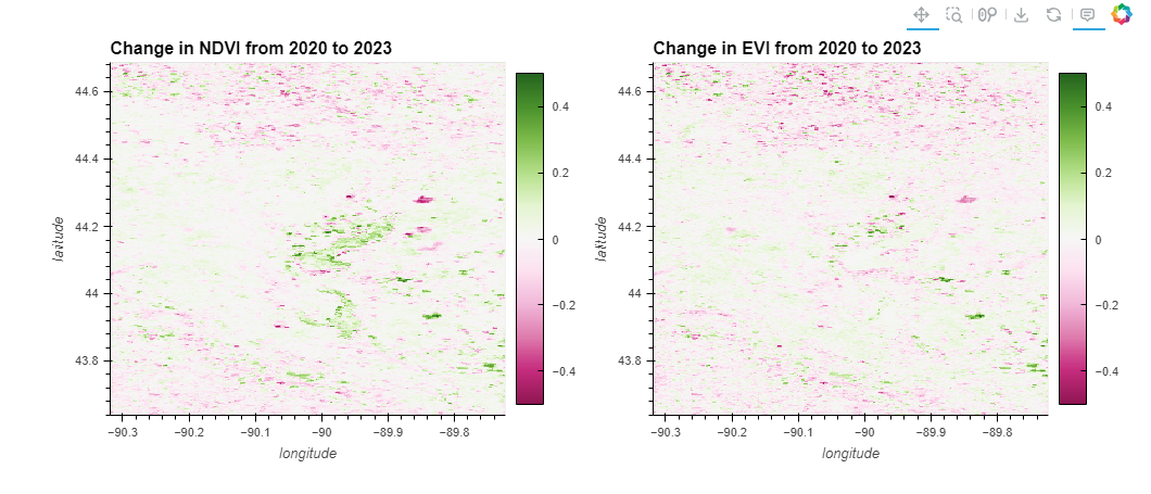
#Debugged code 

# Assume 'ndvi_da' and 'evi_da' are xarray.Dataset objects
# First, let's check and print the structure of these datasets to understand the coordinate names
print(ndvi_da)
print(evi_da)

# Assuming that 'NDVI' and 'EVI' are data variables in your datasets
# Calculate the change in NDVI and EVI over the period
# Replace 'x' and 'y' with actual coordinate names based on the structure printout
ndvi_change = (ndvi_da['NDVI'].sel(date='2023').mean('date') - ndvi_da['NDVI'].sel(date='2020').mean('date'))
evi_change = (evi_da['EVI'].sel(date='2023').mean('date') - evi_da['EVI'].sel(date='2020').mean('date'))

# Check if 'x' and 'y' are appropriate, or if they need to be replaced with 'longitude' and 'latitude'
if 'longitude' not in ndvi_change.coords:
    if 'x' in ndvi_change.coords and 'y' in ndvi_change.coords:
        ndvi_change = ndvi_change.rename({'x': 'longitude', 'y': 'latitude'})
    else:
        # Fallback if no appropriate coordinates are found, you might need to adjust these manually
        print("Appropriate coordinates not found in NDVI dataset")

if 'longitude' not in evi_change.coords:
    if 'x' in evi_change.coords and 'y' in evi_change.coords:
        evi_change = evi_change.rename({'x': 'longitude', 'y': 'latitude'})
    else:
        # Fallback if no appropriate coordinates are found, you might need to adjust these manually
        print("Appropriate coordinates not found in EVI dataset")

# Interactive plotting using hvplot
ndvi_plot = ndvi_change.hvplot.image(x='longitude', y='latitude', cmap='PiYG', clim=(-0.5, 0.5), width=500, height=400, colorbar=True, title='Change in NDVI from 2020 to 2023')
evi_plot = evi_change.hvplot.image(x='longitude', y='latitude', cmap='PiYG', clim=(-0.5, 0.5), width=500, height=400, colorbar=True, title='Change in EVI from 2020 to 2023')

# Display the plots
ndvi_plot + evi_plot

<xarray.Dataset>
Dimensions:      (x: 286, y: 502, date: 12)
Coordinates:
    band         int64 1
  * x            (x) float64 -90.32 -90.32 -90.31 ... -89.73 -89.73 -89.72
  * y            (y) float64 44.68 44.68 44.68 44.68 ... 43.65 43.64 43.64 43.64
    spatial_ref  int64 0
  * date         (date) datetime64[ns] 2020-05-24 2020-06-09 ... 2023-06-26
Data variables:
    NDVI         (date, y, x) float32 0.7044 0.7176 0.6629 ... 0.555 0.555
<xarray.Dataset>
Dimensions:      (x: 286, y: 502, date: 12)
Coordinates:
    band         int64 1
  * x            (x) float64 -90.32 -90.32 -90.31 ... -89.73 -89.73 -89.72
  * y            (y) float64 44.68 44.68 44.68 44.68 ... 43.65 43.64 43.64 43.64
    spatial_ref  int64 0
  * date         (date) datetime64[ns] 2020-05-24 2020-06-09 ... 2023-06-26
Data variables:
    EVI          (date, y, x) float32 0.5624 0.5019 0.5187 ... 0.3659 0.3659

💡Point to Note

💡Strategic Approaches to NDVI and EVI Change Detection Analysis and Anomaly Detection with enhanced Data Handling techniques

The First block code aimed to visualize changes in NDVI and EVI from 2020 to 2023 using hvplot on xarray datasets. However, an error occurred because the data coordinates were not correctly specified or did not exist under the names used in the plotting function ('longitude' and 'latitude'). This is a common issue when working with geospatial data in xarray where coordinate names may vary or be missing, leading to the DataError.

Explanation of the Error: The error message DataError: xarray Dataset must define coordinates for all defined kdims, [Dimension('longitude'), Dimension('latitude')] coordinates not found. indicates that the expected geographic coordinates (longitude and latitude) were not found in the datasets used for plotting. This happens when:

• The dataset uses different names for these dimensions.
• The geographic coordinates are not defined at all, possibly due to the data not being georeferenced properly.
• The coordinate data is present but under different names, like ‘x’ and ‘y’.

Steps to Overcome the Error:

1. Verify Data Structure: First, print the structure of the NDVI and EVI datasets to check the names of the dimensions and coordinates. This helps identify what names are used for what might conventionally be thought of as longitude and latitude.

2. Rename Coordinates: If the coordinates exist but are named differently (e.g., ‘x’ and ‘y’), you can rename them to ‘longitude’ and ‘latitude’ to match the expected names used in the plotting function.

3. Fallback Strategy: If the appropriate coordinates are completely absent, you may need to manually assign these based on your knowledge of the data or handle the absence through other means, such as georeferencing the data if necessary.

Debugged Code Explanation: The debugged code includes checks and renames for the coordinate system to ensure that the plotting function has the correct geographic references. Here’s a breakdown of how the debugged code addresses the issue:

• Check and Rename: The script checks if ‘longitude’ and ‘latitude’ are present in the NDVI and EVI change data. If not, it attempts to find ‘x’ and ‘y’ and renames these coordinates to ‘longitude’ and ‘latitude’.
• Error Handling: It includes print statements to alert the user if the correct coordinates still aren’t found, suggesting that manual adjustments may be needed.
• Visualization: Post-adjustment, the script uses hvplot to visualize the data, ensuring that the geographic dimensions are correctly referenced.

This approach not only fixes the immediate error but also improves the robustness of the script by making it adaptable to datasets with varying coordinate systems. It’s a useful strategy for handling geospatial data where inconsistency in metadata can often lead to errors in processing and visualization.

## Observation 👀🔍

Understanding Vegetation Dynamics through Change Detection Analysis and Anomaly Detection

Change Detection Analysis

Through change detection, shifts in vegetation cover and health over several years are observed. Typically, regions where vegetation has improved or become denser are denoted by green areas in these images, while areas where it has diminished are indicated by pink or red areas. This type of analysis is crucial for the tracking of effects of environmental policies, agricultural practices, and climatic changes on natural and cultivated landscapes.

For example, a particular latitude and longitude point (-89.825, 43.932) from NDVI and EVI analysis with an EVI value of 0.483, indicating vegetation, was examined to determine whether it represents a vegetated area. It was cross-checked with Google Maps by entering the coordinates, and it was found to be an agricultural land area, identifiable by circular patterns in Google Maps.

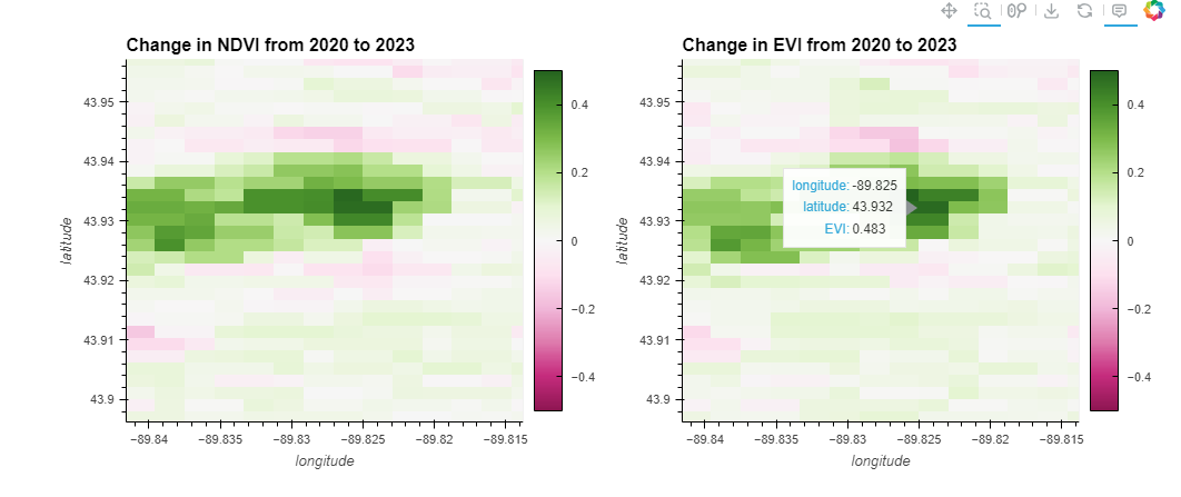
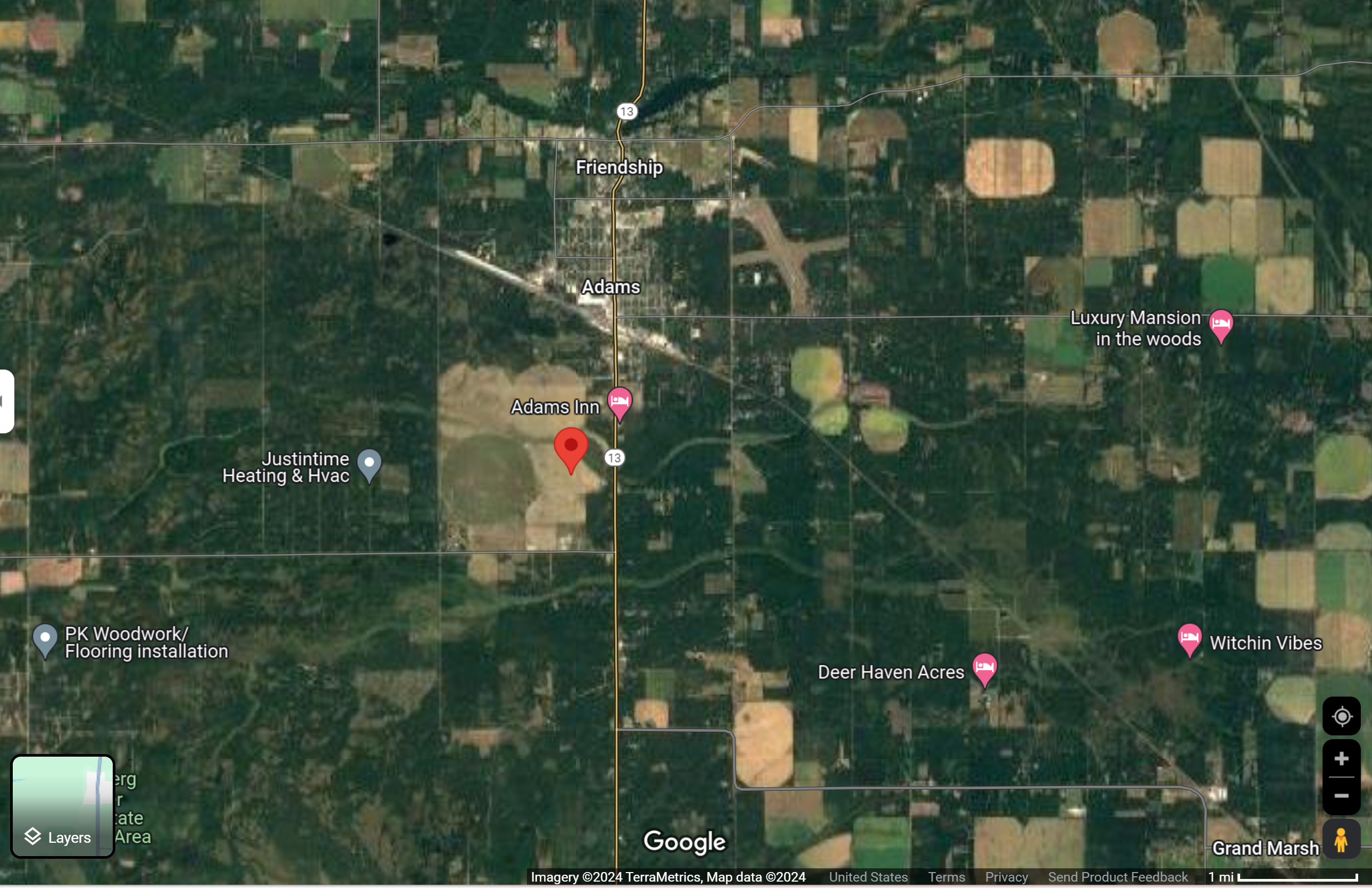
Anomaly Detection

An Interesting Finding: River Appearance in NDVI vs. EVI

One particularly interesting finding in this analysis pertains to the representation of river areas in NDVI and EVI images. While NDVI depicted these water bodies with misleadingly high vegetation signals — shown as continuous green patches — EVI provided a more accurate, subdued portrayal. This anomaly in NDVI often results from its sensitivity to factors other than vegetation, such as reflective surfaces or water turbidity, which can falsely elevate vegetation signals. Conversely, EVI’s formulation, which adjusts for atmospheric and other non-vegetative influences, offers a truer representation, avoiding such distortions and presenting a more reliable depiction of actual vegetation health. This was further validated by checking Google Maps, where this river location was found to be Petenwell Lake in Finley, WI.

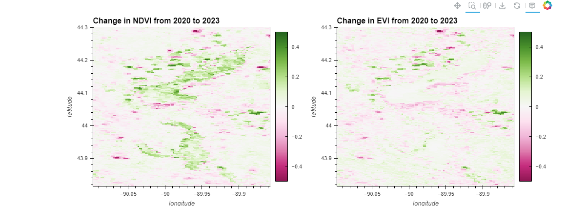
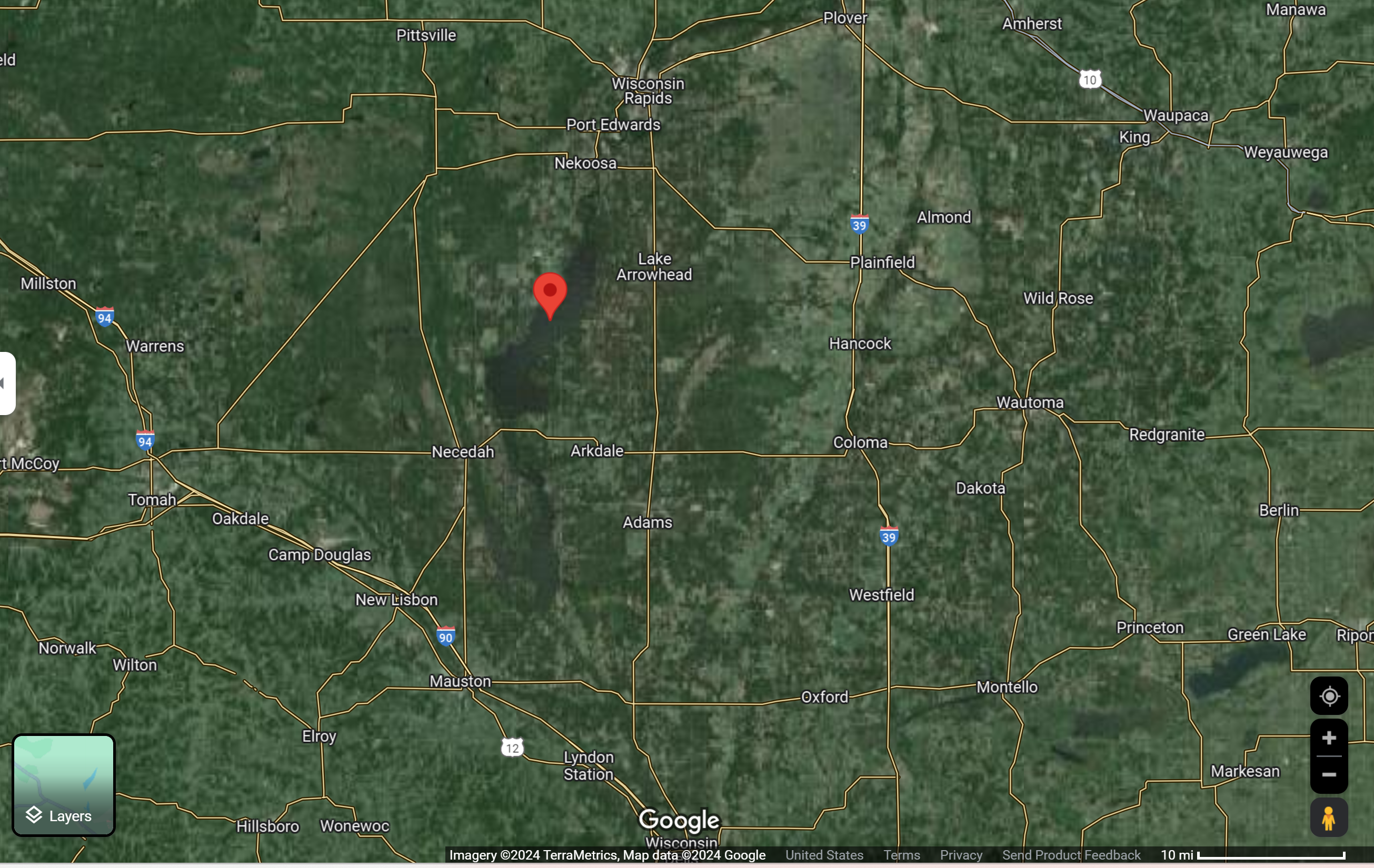
Building on the insights from change detection, anomaly detection serves as a critical follow-up process. This analysis focuses on identifying areas where vegetation indices deviate from expected patterns. In Finley, while some regions showed typical seasonal growth patterns, others displayed unusual anomalies, such as the aforementioned river representation in NDVI. By detecting these anomalies, scientists and environmental managers can pinpoint areas needing further investigation or intervention — perhaps to address pollution impacts, invasive species, or unforeseen environmental stressors.

Anomaly detection not only flags potential errors in data interpretation but also highlights unique or unexpected changes in the ecosystem, guiding more focused studies and informed decision-making. Whether for enhancing agricultural productivity, preserving natural habitats, or planning urban expansion, these tools empower stakeholders with a deeper understanding of the landscape dynamics at play.

🏁Conclusion

Image Source: Satellite Photos are the Earth’s Selfies

This study meticulously explored the dynamic changes in vegetation cover within Finley, WI, through comprehensive analyses using NDVI and EVI indices over a four-year period. Leveraging the power of satellite imagery, the study uncovered temporal and spatial vegetation changes. It demonstrated how to use APIs and strategic approaches in Python Geospatial Programming, along with various analyses involving NDVI and EVI, enabling the creation of real-world applications. This approach could be extended to other geographical locations as well. By applying similar methodologies, researchers and policymakers can gain insights into ecological shifts and the broader impacts of climate change across various ecosystems. Ultimately, the integration of geospatial technologies and dynamic data analysis facilitates more informed decisions in environmental conservation, helping to mitigate the adverse effects of climate change and promoting sustainable development worldwide.

🎯 Final Thoughts

This educational content is a testament to 'Data Driven, Earthly Vision', highlighting the transformative potential of integrating geospatial technology with environmental science. It illustrates how meaningful ecological discoveries and solutions can be driven by advanced analytical tools and data-driven insights. As a learner and practitioner in this field, I am excited to harness the potential of Python geospatial programming and API-driven data analyses to innovate, apply knowledge, and share it with all of you in ways that significantly benefit our planet. Embracing Open and Reproducible Science, we continue to explore and learn—the more we understand our world's natural systems, the better equipped we are to ensure a sustainable and thriving future.

Thank you for reading this article. All the best for your journey in geospatial science, may it be inspiring and fruitful.

This site is open source. Improve this page.